Characterizing Planar Graphs
Vladimir Gudkov, Shmuel Nussinov, Zohar Nussinov

TL;DR
This paper introduces a method for cataloging planar diagrams by utilizing the depth concept, aiming to improve the understanding and classification of planar graphs.
Contribution
It proposes a novel approach to catalog planar graphs based on the depth concept, which is a new perspective in graph theory.
Findings
Effective classification of planar diagrams achieved
Enhanced understanding of planar graph structures
Potential applications in graph visualization and analysis
Abstract
Cataloging planar diagrams using the depth concept is proposed.
Click any figure to enlarge with its caption.
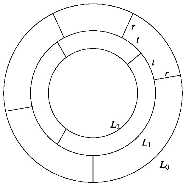 Figure 1
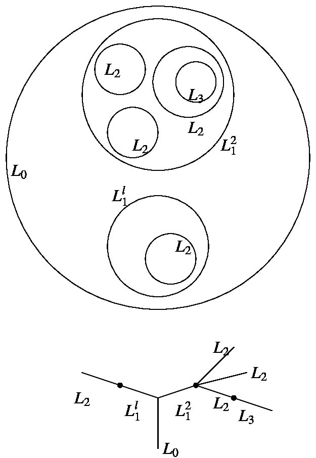 Figure 2
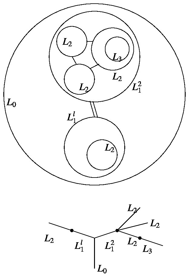 Figure 3
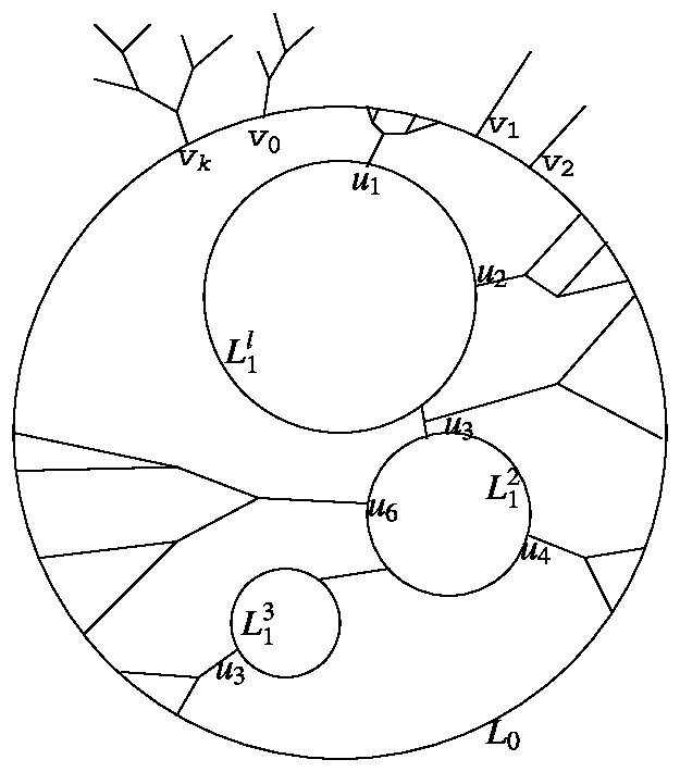 Figure 4
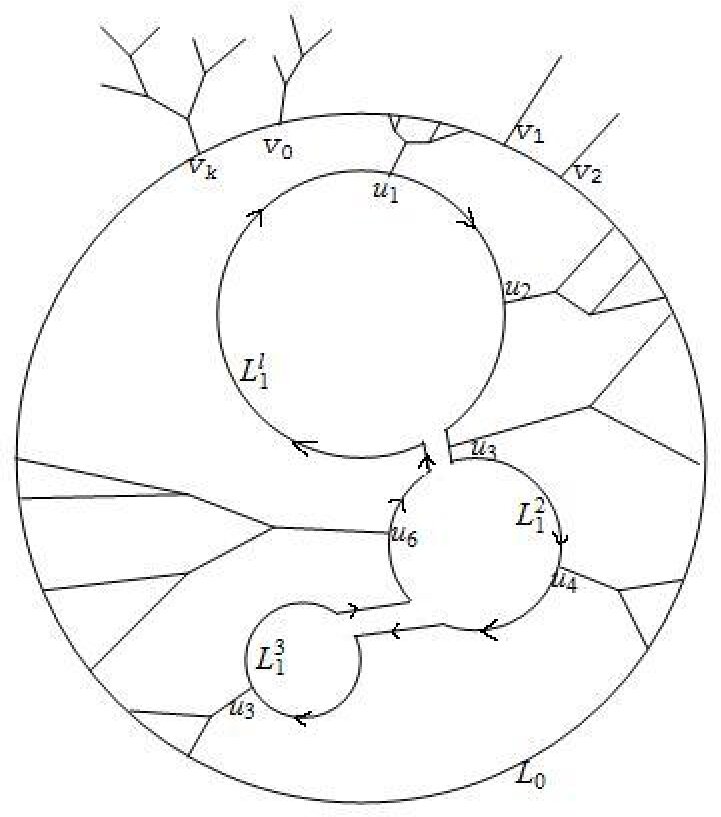 Figure 5
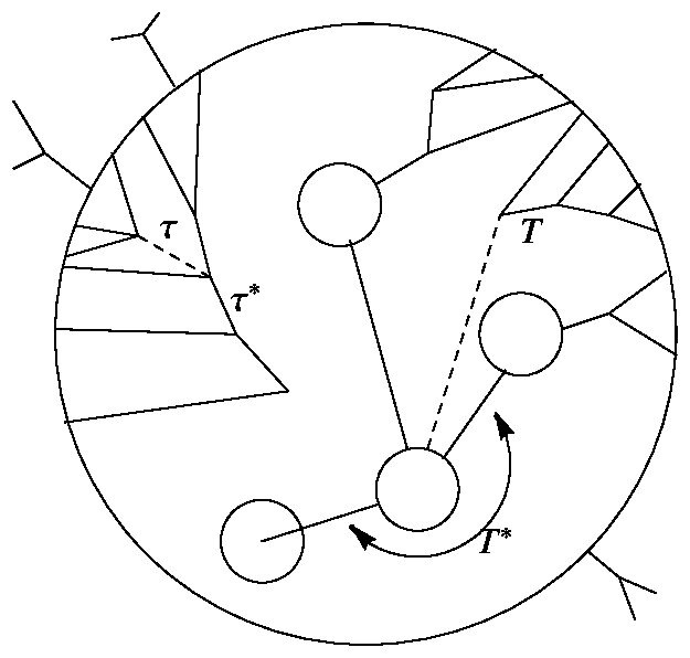 Figure 6
Peer Reviews
No public reviews on file for this paper yet. If you reviewed it on a platform where reviews are public (OpenReview, ICLR, NeurIPS, ICML), you can paste yours below so the community can read it here.
Videos
No videos yet. Explain this paper in a talk, walkthrough, or lecture? Add one.
Taxonomy
TopicsAdvanced Graph Theory Research · Graph Labeling and Dimension Problems · Computational Geometry and Mesh Generation
††thanks: [email protected]††thanks: [email protected]††thanks: [email protected]
Characterizing Planar Graphs
Vladimir Gudkov
Department of Physics and Astronomy, University of South Carolina, Columbia, SC 29208
Shmuel Nussinov
School of Physics and Astronomy, Tel Aviv University, Tel Aviv, Israel
Schmid College of Science, Chapman University, Orange, CA 92866
Zohar Nussinov
Department of Physics, Washington University, St. Louis, Missouri 63160
Kavli Institute for Theoretical Physics, Santa Barbara, CA 93106
Abstract
Cataloging planar diagrams using the depth concept is proposed.
I Introduction
The chararacterization of all graphs is a hard problem. No existing algorithm can test, in polynomial number of steps, if any pair of graphs, represented by adjacency matrices with being the number of vertices, are topologically equivalent.
Planar graphs – namely those graphs which can be drawn on a plane or a sphere without crossing of any two edges – are a special, simple subclass of graphs. Testing for planarity, for equivalence of two planar diagrams, and finding Hamiltonian paths on a planar graph (paths in which each vertex of the graph is visited once and only once) can all be done in polynomial time. Also, simple algorithms transcribed into codes prescribing the construction of any planar graph exist in the mathematical literature NogaAlon .
Here, we characterize planar graphs using a more “physical” approach based on the concept of depth to be defined below.
Interest in planar Feynman diagrams in the high energy community was motivated by ’t-Hooft’s realization 'tHooft:1974pg that in the large limit of non-abelian gauge theories, planar diagrams dominate. More recently, these have been the focus of interest in the condensed matter community. sung-sik Diagrams which can be drawn without crossings only on a surface of genus are in a expansion. The fact that the total number of planar graphs (or finite genus ) increases only as ( rather than as ) was found Koplik:1977pf by using the mathematical literature (mainly by Tutte) on triangulations or by directly solving a zero dimensional field theory Brezin:1977sv . More recently, planar graphs were used in slightly more intricate limits with fermions in appropriately chosen representations in addition to the gauge bosons in Armoni:2003fb .
Explicit summation of all planar diagrams and exact solutions have been achieved only in the dimensional case by ’t-Hooft 'tHooft:1974hx using the fact that only iterated rainbow diagrams contribute to the quark propagator. Further characterizations of planar diagrams may help actual computations.
Mesoscopic devices or printed circuits with predominantly intra (single) plane connections, and highway systems, are also almost planar and characterization of these by depth may be helpful.
II Generalities and the Depth in Planar Graphs
The connectivity, distance, diameter, valency, and other basics can be defined for any graph. The concept of depth defined next is, however, unique to planar graphs. For simplicity, we consider planar diagrams, namely, allow only valency vertices. Lets start with a diagram in coordinate space with no external lines drawn on a sphere. We allow one vertex to have an arbitrary valency, move it to the north pole, and stereographically project on the plane. The special point will be at infinity and the lines from it become the external lines or particles coming from (going to) infinity.
In general, graphs with self energy and tadpole insertions correspond to several different planar drawings. To simplify, we will assume that our graphs are tadpole free and without self energies.
The region around the special vertex (i.e., the point of infinity) is the “exterior” of the graph. The various adjacent “faces” of the graph are divided into classes according to “depth.” The depth of a face is the minimal number of edges that need to be cut in order to reach it from the exterior.
In a “dramatic” description we view the edges in the planar drawing as the walls of a city besieged by outside enemies. Each edge is the boundary between two faces of depths and . The corresponding wall, or edge, is assigned a height
[TABLE]
or
[TABLE]
At each stage, the enemy – or a rising sea encircling our island city – scales (rises above) all walls of given height . Next, it rises to height , etc. Thus, at each stage, the ocean rises by one extra unit and floods faces one unit deeper.
III Going from One Depth to the Next
The gradual flooding process allows peeling off successive layers of the besieged island or eventually of each of the separate islands previously generated. This allows a recursive definition of the complete graph.
Edges of type (1) or (2) above, are termed “tangential” or “radial” respectively, a nomenclature suggested by the special graph with concentric circles threaded by radial “spokes” emanating from the center (see Fig. 1).
The tangential edges contribute to the defense of our island from the steadily rising sea, whereas radial edges, needed for the connectivity of the graph, do not help this defense at all. Thus the two faces flanking a radial edge have equal depths and get flooded simultaneously. On the other hand, any tangential edge of type (1) separates two faces of depths differing by one unit. Hence, once the lower depth face is flooded, the tangential wall in question still protects the “inner,” deeper face. A series of contiguous tangential edges separates an “outer” region of depth from an “inner” region of depth . At some point, the depth faces will all be flooded by the “ocean” which constitutes one continuous connected body of “water.” Hence, the chain of contiguous tangential edges cannot be terminated at a vertex. In such a case, the ocean would have “flanked” this chain on both sides, and the chain cannot separate two regions. The boundary of any region has no boundary and a continuous chain of tangential line must form a closed “circular” loop.
In general, the complete set of tangential lines defending regions of a given depth form several disconnected loops, each enclosing a separate “island” which is a smaller subgraph of the original graph. An important simplifying feature is that these inner planar subgraphs – being physically separated from the outside region, and from each other – can be independently prescribed. This is the key to our recursive definition. The main steps involved amount to repeated constructions either of actual tree subgraphs or using “tree like” combinatorics.
Consider first the “overall” depth structure of the graph as manifest by drawing all the closed loops encircling the islands arising at all the stages of the flooding process. These consist of the large overall boundary encircling the complete graph of depth . Inside this loop, we have one or up to separate loops each encircling a subgraph of depth . Inside each of the above “first generation” loops, we have one or several loops, all together adding up to “second generation” loops, etc ( see Fig. 2).
This hierarchy of inclusions is tree-like. Thus, consider a real physical tree growing vertically and dividing into branches, each branch next divides into branches of the next generation, etc. By cutting the full tree at each of the levels and projecting all cuts, we generate exactly the original hierarchical set of loops made up of all the tangential edges. The equivalent – in this case, a rather simple “tree of loops” – is illustrated at the bottom of Fig. 2.
We still have to construct the remaining set of “radial” edges in the region between an “external” loop around a region of depth and in general several smaller “inner” loops each encircling a subgraph of depth .
This construction repeats itself at each depth or generation. We start with the complete original diagram but will keep in mind also the analog repeats in later generations. The external lines can merge into trees , , , with having tips, so that . The trees are “rooted” along the overall encircling loop at vertices as indicated in Fig. 4 bellow. For concreteness, we define one such vertex as and number the rest in a clockwise direction. These external vertices then carry the complete information pertinent for all subsequent steps performed inside as described below, which is inherited from the outside.
Consider next the loops encircling islands of depth , which are exposed after the outside big loop eroded. We can connect those to each other via “radial” edges. We should not connect two loops by more than one line. Otherwise, rather than having two different circular loops, they will be joined to one bigger circular loop. More generally, we should not form bigger new type loops in the next generation using the new lines and portions of the above loops (see e.g. Fig. 3).
Otherwise, this bigger loop, rather then the individual smaller loops, will be exposed after the first stage. Thus, we can only connect the loops by single lines into one overall “tree” (whose vertices are the above loops) or to several separate such trees (see Fig. 4).
Apart from partitioning the loops into the subsets forming the vertices of these trees, we have again just tree formation.
Next, we add radial edges joining the above trees of loops to the outer big overall loop. Some such edges are needed to ensure connectivity. To avoid modifying the first generation circular loop(s), the connection to the “outer frame” should be only via trees rooted on the inner loops with tips on the outer loop. These trees are similar to what we assumed above for the external lines forming trees that are attached from the outside to the external loop. Indeed, by construction, the trees offer no further defense when the outside big loop is stripped off, conforming to the definition of radial edges of which these trees are made. Being directly parts of the graph, the assumed threefold valency implies that these are simple binary trees. There is still the question of how to place the tree tips from the inside between the tree roots from the outside without violating the required planarity.
We start first with the simple case with just one inner loop. There are special points on both the external and internal loops, namely, the roots of the external particle trees and the roots of the internal trees . Each “first generation” tree, maps, via its tips, the -th point on the internal loop to an interval on the outer loop where all the tips reside. Each interval is flanked by two external points and with being the number of external points in this interval. In the case when for all : if , we have no line crossings of edges of the different trees and planarity can be maintained.
By assumption all the first generation loops are connected so as to form a single tree of loops. We will denote such “trees of loops” by ’s and the “true” binary trees connecting them to the external loop by ’s. Next – just for the purpose of ordering the vertices – we imagine doubling the lines connecting the tree of loops (see Fig. 5). This induces a common clockwise ordering111 This is the case for graphs drawn on orientable manifold including higher Genus surfaces. of all the vertices and the trees emanating from the various loops and possibly also from the connecting lines.
The first generation loops can form several (say ) disconnected “trees of loops” , , with the roots of the “real” binary trees residing on the loops (or connecting lines); and each of the trees of loops can separately be clock-wise ordered as above. We then have binary trees rooted on the first generation loops or on the lines between those and connected to the external overall loop.
In addition we can have some number of “hanging” binary trees attached only to the external loop. The last stage of defining the recursive process of going from depth to depth involves placing the tips of the above , first (-th in general) generation trees relative to roots of exterior (in general -th generation) trees on the surrounding big loop. This involves further combinatoric which we discuss in the next section.
IV The ”Tree” of the Nesting Hierarchy of Trees
Connecting the tips of the first ( -th) generation trees to the external (-th generation) loop again involves “tree like” constructions.
Any of these trees can be “nested” within consecutive branches of another tree, and other trees can be nested between pairs of its branches. The “lowest”in this hierarchy are trees which harbor no other trees. The tips of any of these “non-harboring” trees, , define a continuous single interval on the exterior encircling loop on which all its tips reside. (This interval must contain at least one root of the external trees or, more generally, a root of a tree from a previous generation. Otherwise, the tree hangs from one tangential edge making a “mass” insertion which was excluded by assumption). One notch higher in the nestling hierarchy are trees which nestle lowest echelon of trees, ’s . Two tips of should land on the external ring on the two sides of the interval associated with the nestled tree ’s. Recall that the interval contains all the tips of the tree . This should be the case for all intervals corresponding to all trees nestled within . All these intervals together with the tips of then cover a larger continuous interval , the overall domain of influence of the harboring tree . In turn, several such ’s and possibly an additional first echelon of trees ’s nestle within yet a higher (in nestling hierarchy) tree , etc. This can keep on going until all the radial edges composing trees connecting the -th generation loops to the encircling single -th generation loop are exhausted. To specify fully the nestling, we need not only to know which tree is a given tree nested in, but also to specify the two branches between which the lower echelon is nested, as is the case here with a tree. As indicated in Fig. 6, it is specified by an extra “pointer edge” (shown as a broken line) connecting the branching point of the tree and the root of the tree nested therein.
Thus, to specify fully the set-up bridging between two consecutive depths, we formally need an extra “field” , whose propagator is the above broken line (as opposed to the propagator of the main field denoted by the full edges in the diagram) and also, in addition to the true vertices of the original graph, some vertices to allow the above pointers.
Finally, in this nestling process, we cannot treat the hanging trees and the loop () trees the same way.
When nested within a higher echelon tree, the whole tree of loops along with the many ordinary -type trees spawned off from it are both treated as one nested unit. Still, we need to maintain the correct ordering on the external loop the of the trees spawned from the loops of the trees, and the correct cyclic ordering relative to the external loops above has to be maintained.
Further, when nesting trees within a higher echelon trees, the and trees are also clearly different. The point is that each tree “spawns” several regular trees, and we need to specify in which tree (we are using the broken line indicators for these specific junctions) is the tree is nested.
The process of defining successively broader domains of influence on the external loop, each containing contiguous domains of influence of lower hierarchy trees, is clearly isomorphic to building a general “nestling tree” and even pictorially is similar to the basic tree made of tangential loops of higher depth (Fig. 3). There, the largest, most inclusive, outermost loop is indeed the root of the abstract inclusion tree. Here, there is some ambiguity as to which tree provides the root of the “nestling hierarchy tree”: we can sometimes declare that tree is nested within or, reversing the point of view, that is nested within . We avoid this ambiguity by using the ”origin,” namely, the first vertex on the external loop. It will induce the ”origins” on each of the internal loops, namely the point on each loop closest to it in a clock wise sense. We declare the overall nestling tree – the one highest in the hierarchy of nesting (encountered in any of the depth= depth= transition) – to be the one whose domain of influence includes the origin on the encircling loop.
V Summary and Further Comments.
The above recursive definition of the general planar graph by means of the concept of depth is clearly not the simplest or the most concise possible. In such terms, it is significantly inferior to the concise formal mathematical construction. We hope, however, that this particular method, being based on a heuristic “physical” notion of depth, may be useful in some physical applications. Specifically, in computing planar Feynman diagrams, it is interesting to ask if the tangential loops and radial trees can offer a more natural way for routing the momenta. (The question as to the optimal “choice of loops” occurs already for electrical networks.) Thus, rather than using the individual elementary faces of the planar graph for the loops, we can use the “circular” loops made of “tangential” edges. All the external moments (or currents) can then be made to flow only in the external overall loop. It is often the case that the sum of one loop diagrams with any number of external lines defines a useful effective action. By envisioning that the planar diagrams are in configuration space we may have here effective actions on different scales. Then, the effective actions of larger and larger circular loops may correspond to steps in a renormalization group that begin with short distances and then build up the exact (in the planar approximation) infrared physics.
The fact that all the combinatorics involved in our construction of the diagrams was essentially of repeated construction of trees suggests, at different levels of abstractions that there may be some reasonably simple semi classical description.
VI Acknowledgements
We are indebted to Noga Alon for very useful discussions of the above subject and other graph connected issues.
The reference list from the paper itself. Each links out to its DOI / PubMed record.
- 1(1) Private communication from Noga Alon.
- 2(2) G. ’t Hooft, Nucl. Phys. B 72 , 461 (1974).
- 3(3) Sung-Sik Lee, ar Xiv:cond-mat/0905.4532 (2009)
- 4(4) J. Koplik, A. Neveu and S. Nussinov, Nucl. Phys. B 123 , 109 (1977).
- 5(5) E. Brezin, C. Itzykson, G. Parisi and J. B. Zuber, Commun. Math. Phys. 59 , 35 (1978).
- 6(6) A. Armoni, M. Shifman and G. Veneziano, Phys. Rev. Lett. 91 , 191601 (2003) [ar Xiv:hep-th/0307097].
- 7(7) G. ’t Hooft, Nucl. Phys. B 75 , 461 (1974).