Mutant knots and intersection graphs
S.V.Chmutov, S.K.Lando

TL;DR
This paper investigates the relationship between mutant knots, intersection graphs, and weight systems, showing that invariants insensitive to mutation depend only on intersection graphs, with implications for Lie algebra weight systems.
Contribution
It establishes a connection between knot invariants, mutant knots, and intersection graphs, highlighting when invariants depend solely on intersection graphs.
Findings
Invariants not distinguishing mutants depend on intersection graphs.
The converse that such invariants depend on diagrams is well known.
Discusses links to Lie algebra weight systems.
Abstract
We prove that if a finite order knot invariant does not distinguish mutant knots, then the corresponding weight system depends on the intersection graph of a chord diagram rather than on the diagram itself. The converse statement is easy and well known. We discuss relationship between our results and certain Lie algebra weight systems.
Click any figure to enlarge with its caption.
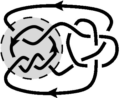 Figure 1
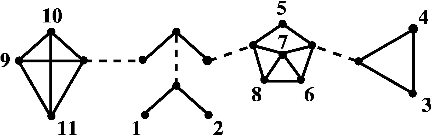 Figure 2
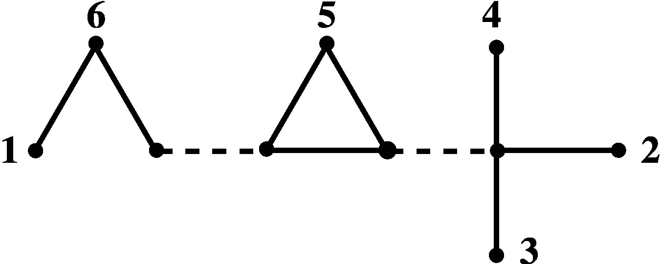 Figure 3
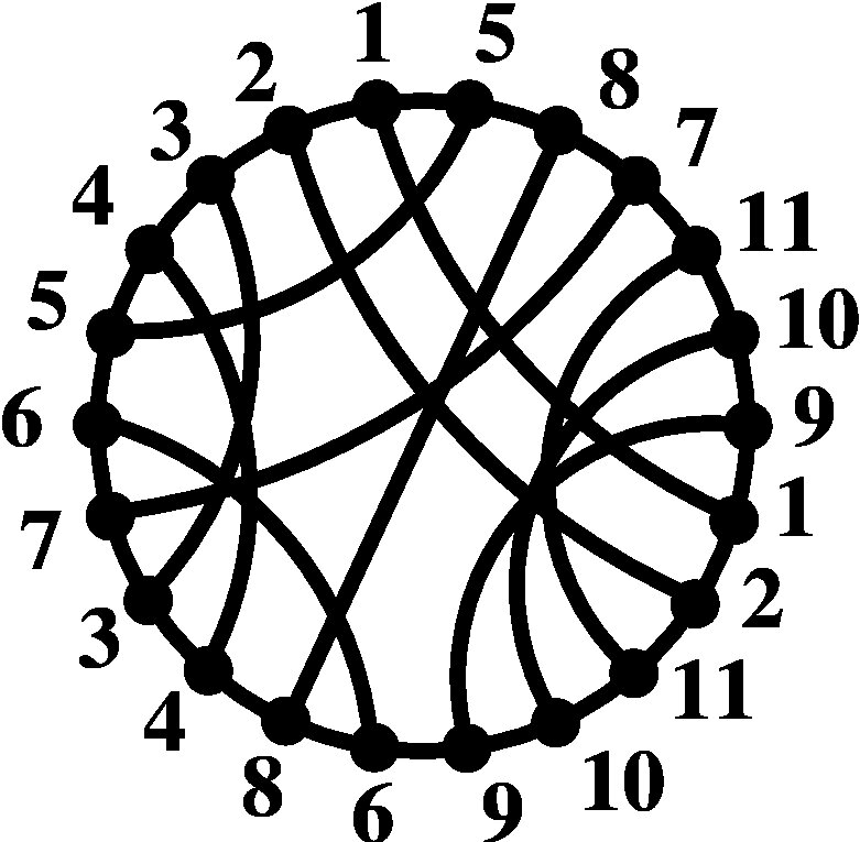 Figure 4
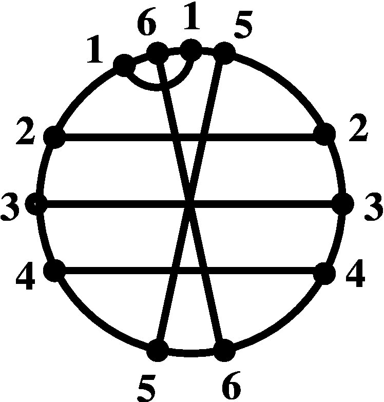 Figure 5
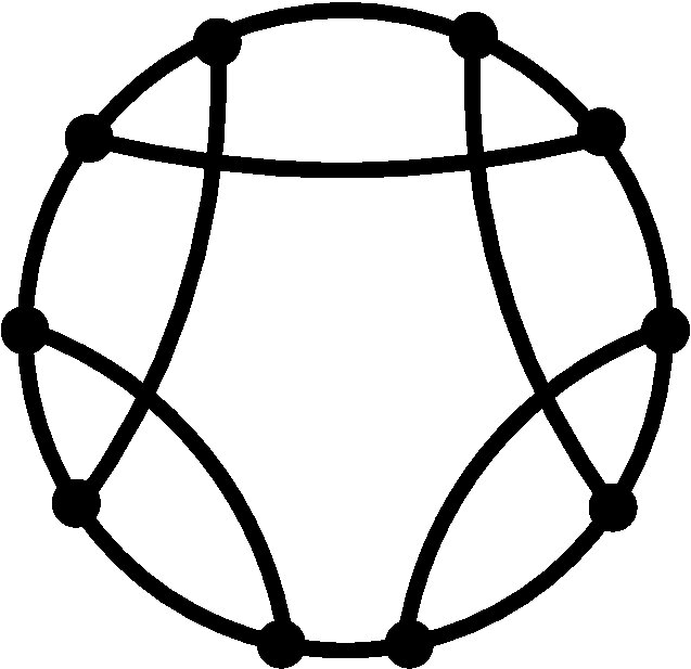 Figure 6
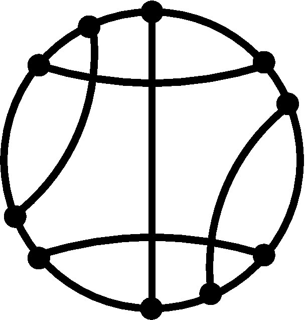 Figure 7
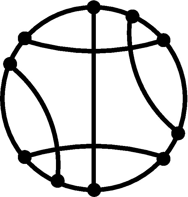 Figure 8
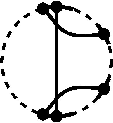 Figure 9
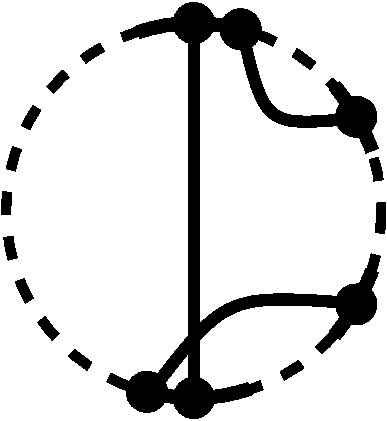 Figure 10
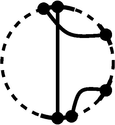 Figure 11
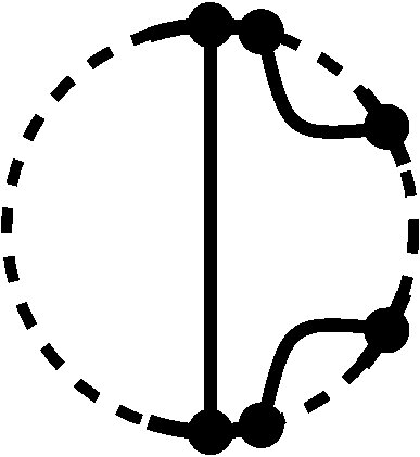 Figure 12
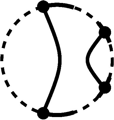 Figure 13
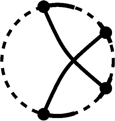 Figure 14
 Figure 15
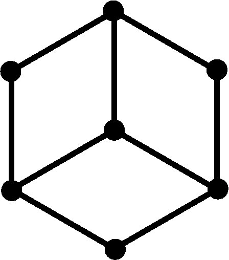 Figure 16
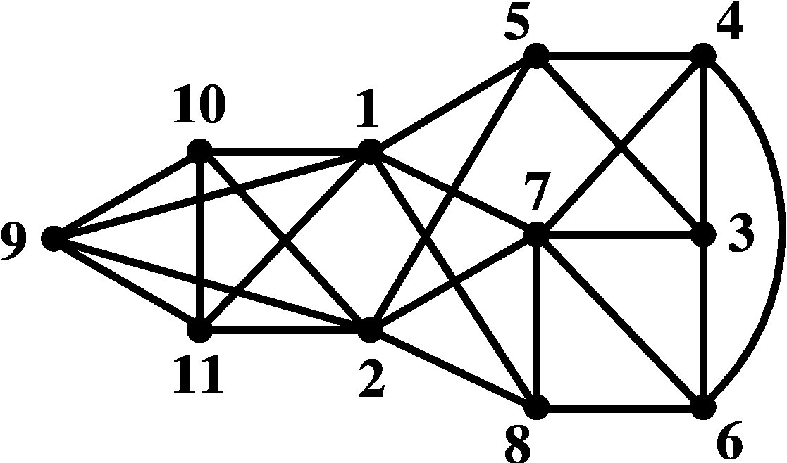 Figure 17
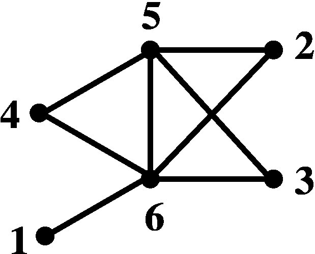 Figure 18
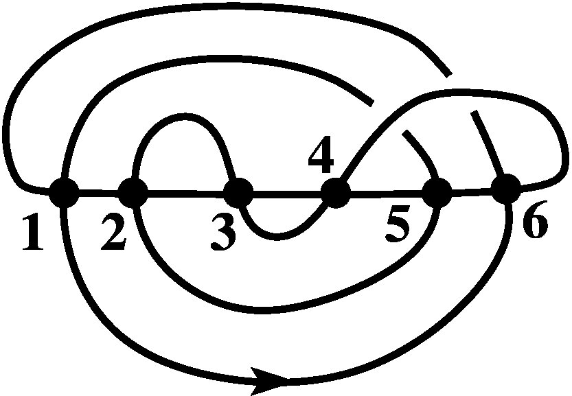 Figure 19
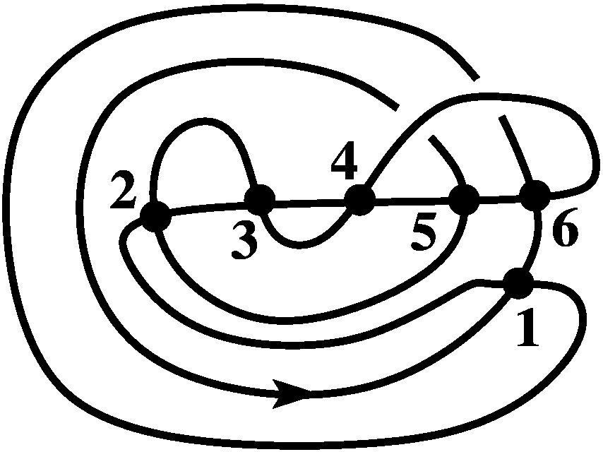 Figure 20
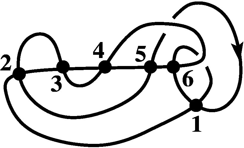 Figure 21
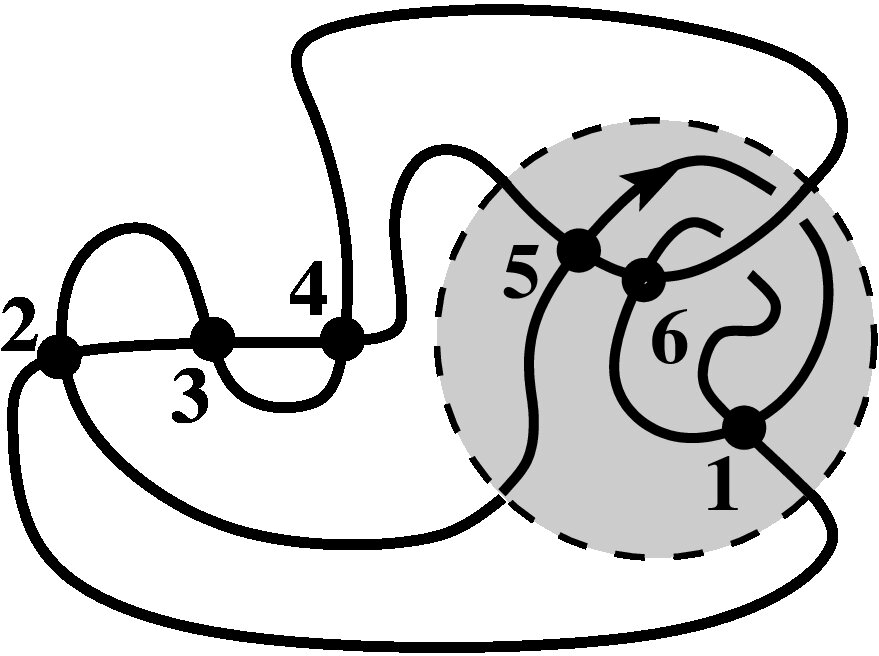 Figure 22
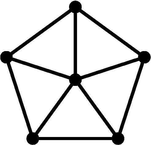 Figure 23
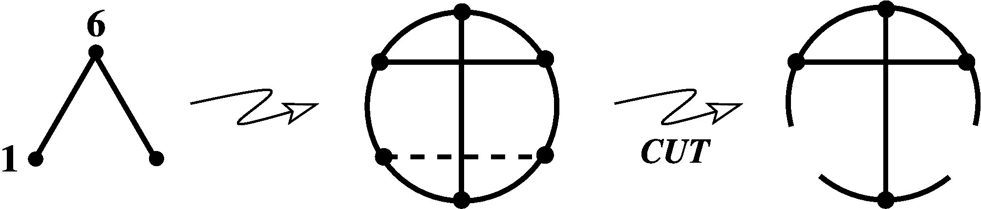 Figure 24
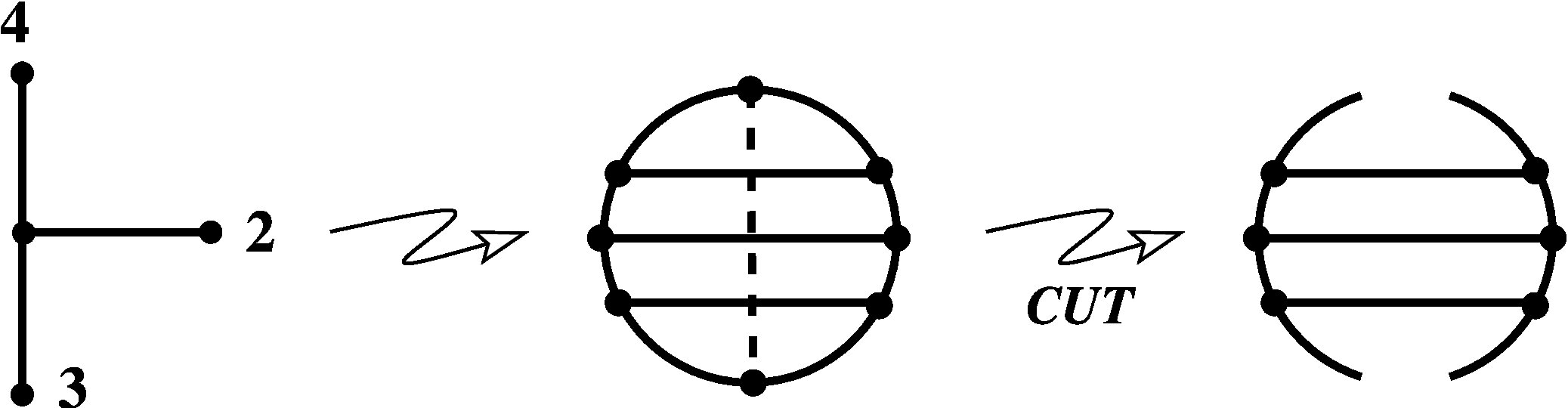 Figure 25
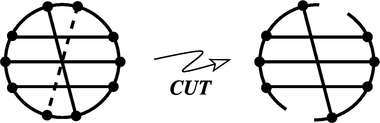 Figure 26
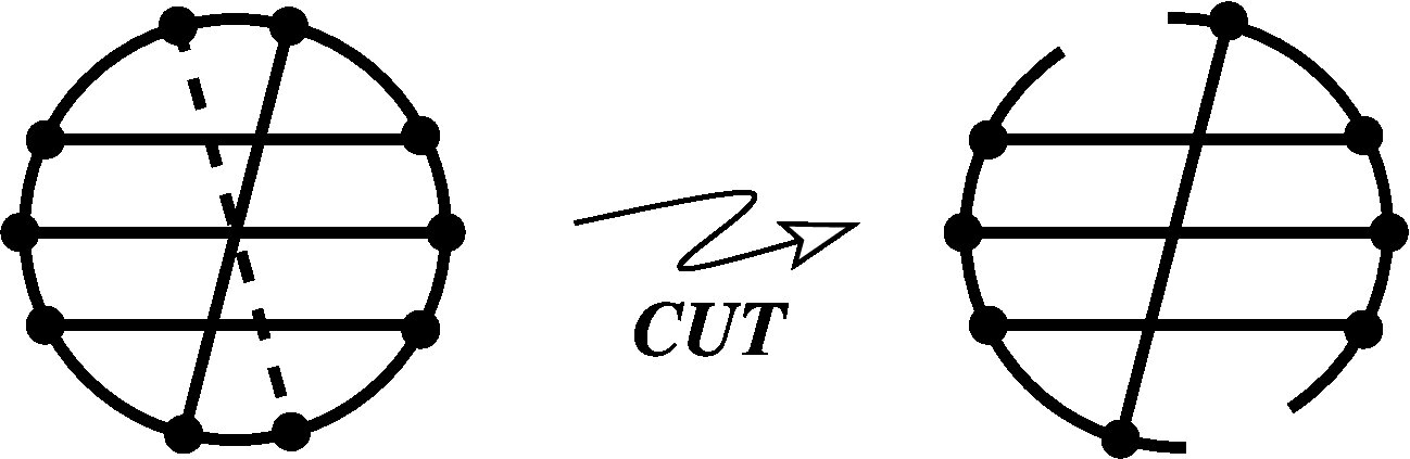 Figure 27
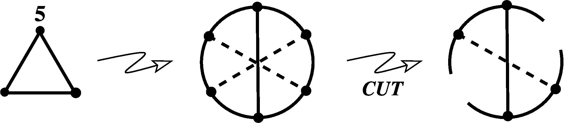 Figure 28
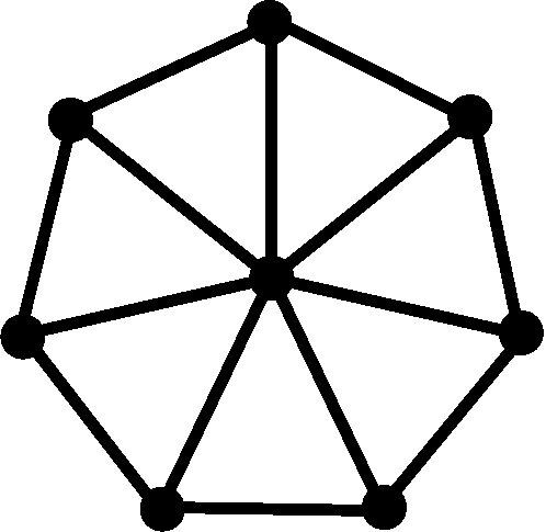 Figure 29
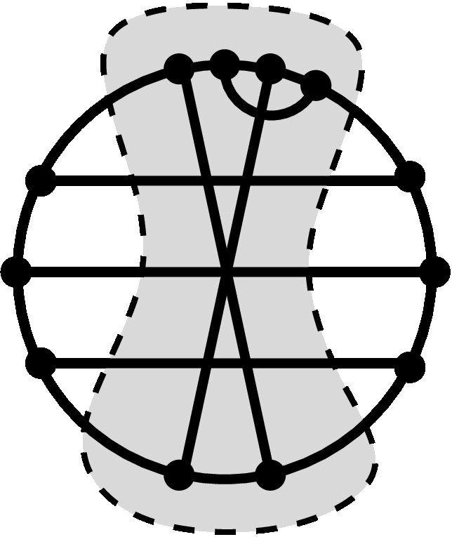 Figure 30
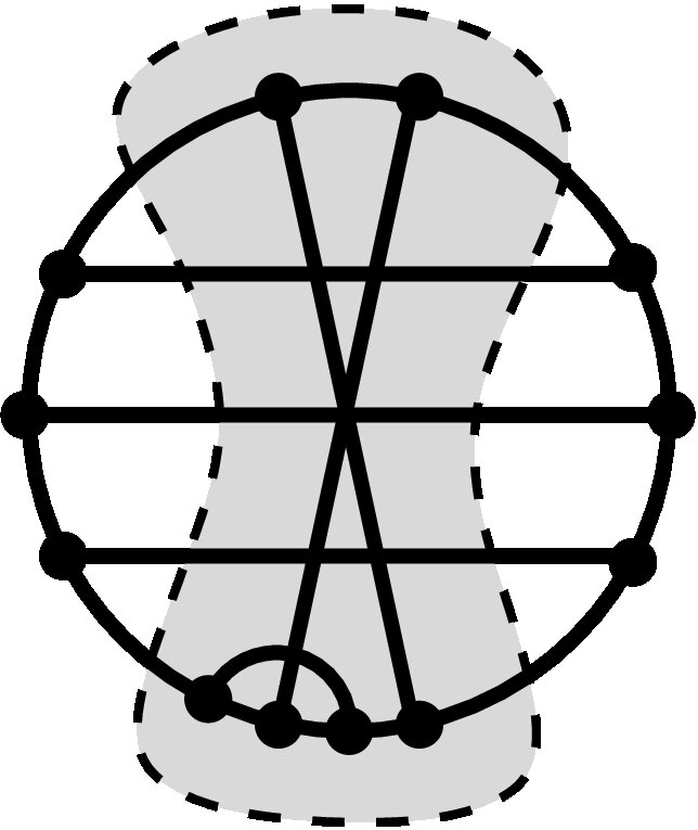 Figure 31
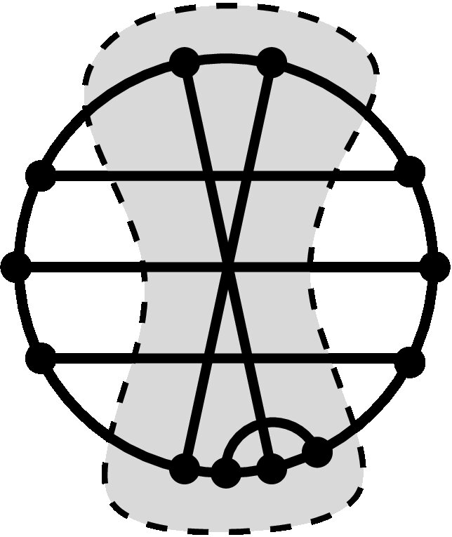 Figure 32
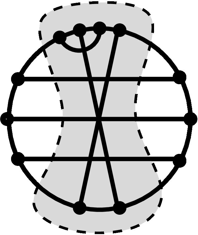 Figure 33
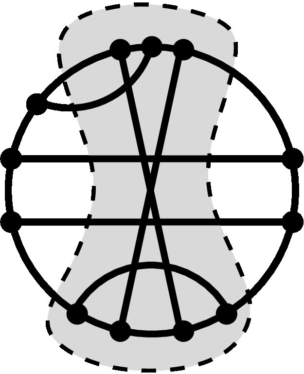 Figure 34
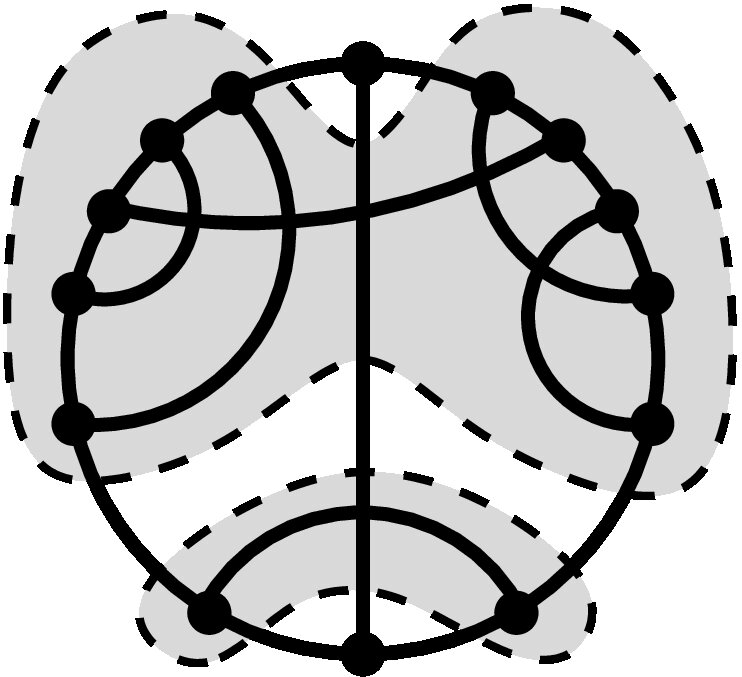 Figure 35
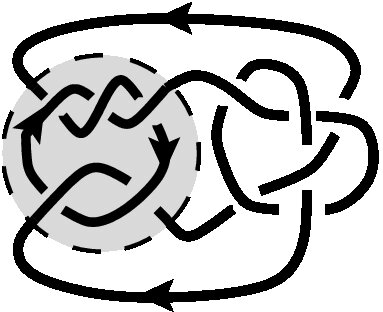 Figure 36
Peer Reviews
No public reviews on file for this paper yet. If you reviewed it on a platform where reviews are public (OpenReview, ICLR, NeurIPS, ICML), you can paste yours below so the community can read it here.
Videos
No videos yet. Explain this paper in a talk, walkthrough, or lecture? Add one.
Mutant knots and intersection graphs
S. V. Chmutov, S. K. Lando The Ohio State University, Mansfield.Institute for System Research RAS and the Poncelet Laboratory, Independent University of Moscow, partly supported by the grant ACI-NIM-2004-243 (Noeuds et tresses), RFBR 05-01-01012-a, NWO-RFBR 047.011.2004.026 (RFBR 05-02-89000-NWOa), GIMP ANR-05-BLAN-0029-01.
(April 10, 2007)
Abstract
We prove that if a finite order knot invariant does not distinguish mutant knots, then the corresponding weight system depends on the intersection graph of a chord diagram rather than on the diagram itself. The converse statement is easy and well known. We discuss relationship between our results and certain Lie algebra weight systems.
1 Introduction
Below, we use standard notions of the theory of finite order, or Vassiliev, invariants of knots in -space; their definitions can be found, for example, in [6] or [14]. All knots are assumed to be oriented.
Two knots are said to be mutant if they differ by a rotation/reflection of a tangle with four endpoints; if necessary, the orientation inside the tangle may be replaced by the opposite one. Here is a famous example of mutant knots, the Conway () knot of genus 3, and Kinoshita–Terasaka () knot of genus 2 (see [1]).
[TABLE]
Note that the change of the orientation of a knot can be achieved by a mutation in the complement to a trivial tangle.
Most known knot invariants cannot distinguish mutant knots. Neither the (colored) Jones polynomial, nor the HOMFLY polynomial, nor the Kauffman two variable polynomial distinguish mutants. All Vassiliev invariants up to order 10 do not distinguish mutants as well [17] (up to order 8 this fact was established by a direct computation [5, 6]). However, there is a Vassiliev invariant of order 11 distinguishing and [16, 17]. It comes from the colored HOMFLY polynomial.
The main combinatorial objects of the Vassiliev theory of knot invariants are chord diagrams. To a chord diagram, its intersection graph (also called circle graph) is associated. The vertices of the graph correspond to chords of the diagram, and two vertices are connected by an edge if and only if the corresponding chords intersect.
The value of a Vassiliev invariant of order on a singular knot with double points depends only on the chord diagram of the singular knot. Hence any such invariant determines a function, a weight system, on chord diagrams with chords. Conversely, any weight system induces, in composition with the Kontsevich integral, which is the universal finite order invariant, a finite order invariant of knots. Such knot invariants are called canonical. Canonical invariants span the whole space of Vassiliev invariants.
Direct calculations for small show that the values of these functions are uniquely determined by the intersection graphs of the chord diagrams. This fact motivated the intersection graph conjecture in [5] (see also [6]) which states that any weight system depends on the intersection graph only. This conjecture happened to be false, because of the existence of a finite order invariant that distinguishes two mutant knots mentioned above and the following fact.
The knot invariant induced by a weight system whose values depend only on the intersection graph of the chord diagrams cannot distinguish mutants.
A justification of this statement, due to T. Le (unpublished), looks like follows (see details in [6]). If we have a knot (in general position) with a distinguished two-string tangle, then all the terms in the Kontsevich integral of the knot having chords connecting the tangle with its exterior vanish.
Our goal is to prove the converse statement thus establishing an equivalence between finite order knot invariants nondistinguishing mutants and weight systems depending on the intersection graphs of chord diagrams only.
Theorem 1
If a finite order knot invariant does not distinguish mutants, then the corresponding weight system depends only on the intersection graphs of chord diagrams.
Together, the two statements can be combined as follows.
A canonical knot invariant does not distinguish mutants if and only if its weight system depends on the intersection graphs of chord diagrams only.
Recently, B. Mellor [15] extended the concept of intersection graph to string links. We do not know whether our Theorem 1 admits an appropriate generalization.
Section 2 is devoted to the proof of Theorem 1. In Sec. 3, we discuss relationship between intersection graphs and the weight systems associated to the Lie algebra and the Lie algebra .
The paper was written during the second author’s visit to the Mathematical Department of the Ohio State University. He expresses his gratitude to this institution for warm hospitality and excellent working conditions. The authors are grateful to S. Duzhin, K. J. Supowit, and A. Vaintrob for useful discussions.
2 Proof
2.1 Representability of graphs as the intersection graphs
of chord diagrams
Not every graph can be represented as the intersection graph of a chord diagram. For example, the following graphs are not intersection graphs.
[TABLE]
A characterization of those graphs that can be realized as intersection graphs is given by an elegant theorem of A. Bouchet [4].
On the other hand, distinct diagrams may have coinciding intersection graphs. For example, next three diagrams have the same intersection graph :
[TABLE]
A combinatorial analog of the tangle in mutant knots is a share [5, 6]. Informally, a share of a chord diagram is a subset of chords whose endpoints are separated into at most two parts by the endpoints of the complementary chords. More formally,
Definition 1
A share is a part of a chord diagram consisting of two arcs of the outer circle possessing the following property: each chord one of whose ends belongs to these arcs has both ends on these arcs.
Here are some examples:
[TABLE]
The complement of a share also is a share. The whole chord diagram is its own share whose complement contains no chords.
Definition 2
A mutation of a chord diagram is another chord diagram obtained by a rotation/reflection of a share.
For example, three mutations of the share in the first chord diagram above produce the following chord diagrams:
[TABLE]
Obviously, mutations preserve the intersection graphs of chord diagrams.
Theorem 2
Two chord diagrams have the same intersection graph if and only if they are related by a sequence of mutations.
This theorem is contained implicitly in papers [3, 8, 11] where chord diagrams are written as double occurrence words, the language better suitable for describing algorithms than for topological explanation.
**Proof of Theorem 2.
**The proof of this theorem uses Cunningham’s theory of graph decompositions [9].
A split of a (simple) graph is a disjoint bipartition of its set of vertices such that each part contains at least 2 vertices, and there are subsets , such that all the edges of connecting with form the complete bipartite graph with the parts and . Thus for a split the whole graph can be represented as a union of the induced subgraphs and linked by a complete bipartite graph.
Another way to think about splits, which is sometimes more convenient and which we shall use in the pictures below, looks like follows. Consider two graphs and each having a distinguished vertex and , respectively, called markers. Construct the new graph whose set of vertices is
[TABLE]
and whose set of edges is
[TABLE]
Representation of as is called a decomposition of , and are called the components of the decomposition. The partition is a split of . Graphs and might be decomposed further giving a finer decomposition of the initial graph . Pictorially, we represent a decomposition by pictures of its components where the corresponding markers are connected by a dashed edge.
A prime graph is a graph with at least three vertices admitting no splits. A decomposition of a graph is said to be canonical if the following conditions are satisfied:
- (i)
each component is either a prime graph, or a complete graph , or a star , which is the tree with a vertex, the center, adjacent to other vertices;
- (ii)
no two components that are complete graphs are neighbors, that is, their markers are not connected by a dashed edge;
- (iii)
the markers of two components that are star graphs connected by a dashed edge are either both centers or both not centers of their components.
W. H. Cunningham proved [9, Theorem 3] that each graph with at least six vertices possesses a unique canonical decomposition.
Let us illustrate the notions introduced above by two examples of canonical decomposition of the intersection graphs of chord diagrams. We number the chords and the corresponding vertices in our graphs, so that the unnumbered vertices are the markers of the components. The first example is our example from page 2:
[TABLE]
The second example represents the chord diagram of the double points in the plane diagram of the Conway knot from page 1. The double points of the shaded tangle are represented by the chords 1,2,9,10,11.
[TABLE]
The key observation in the proof of Theorem 2 is that components of the canonical decomposition of any intersection graph admit a unique representation by chord diagrams. For a complete graph and star components, this is obvious. For a prime component, this was proved by A. Bouchet [3, Statement 4.4] (see also [11, Section 6] for an algorithm finding such a representation for a prime graph).
Now to describe all chord diagrams with a given intersection graph, we start with a component of its canonical decomposition. There is only one way to realize the component by a chord diagram. We draw the chord corresponding to the marker as a dashed chord and call it the marked chord. This chord indicates the places where we must cut the circle removing the marked chord together with small arcs containing its endpoints. As a result we obtain a chord diagram on two arcs. Repeating the same procedure with a neighbor component of the canonical decomposition, we get another chord diagram on two arcs. We have to sew these two diagrams together by their arcs in an alternating order. There are four possibilities to do this, and they differ by mutations of the share corresponding to the second (or, alternatively, the first) component. This completes the proof of Theorem 2.
To illustrate the last stage of the proof consider our standard example and take the star 2-3-4 component first and then the triangle component. We get
[TABLE]
Because of the symmetry, the four ways of sewing these diagrams produce only two distinct chord diagrams with a marked chord:
[TABLE]
repeating the same procedure with the marked chord for the last 1-6 component of the canonical decomposition, we get
[TABLE]
Sewing this diagram into the previous two in all possible ways we get four mutant chord diagrams from page 2.
As an enjoyable exercise we leave to the reader to work out our second example with the chord diagram of the diagram of the Conway knot and find the mutation producing the chord diagram of the plane diagram of the Kinoshita–Terasaka knot using the canonical decomposition.
2.2 Proof of Theorem 1
Suppose we have a Vassiliev knot invariant of order at most that does not distinguish mutant knots. Let and be chord diagrams with chords whose intersection graphs coincide. We are going to prove that the values of the weight system of on and are equal.
By Theorem 2, it is enough to consider the case when and differ by a single mutation in a share . Let be a singular knot with double points whose chord diagram is . Consider the collection of double points of corresponding to the chords occurring in the share . By the definition of a share, has two arcs containing all these double points and no others. By sliding the double points along one of these arcs and shrinking the other arc we may enclose these arcs into a ball whose interior does not intersect the rest of the knot. In other words, we may isotope the knot to a singular knot so as to collect all the double points corresponding to in a tangle . Performing an appropriate rotation of we obtain a singular knot with the chord diagram . Since does not distinguish mutants, its values on and are equal. Theorem 1 is proved.
To illustrate the proof, let be the chord diagram from our standard example. Pick a singular knot representing , say
[TABLE]
To perform a mutation in the share containing the chords 1,5,6, we must slide the double point 1 close to the double points 5 and 6, and then shrink the corresponding arcs:
[TABLE]
Now doing an appropriate rotation of the tangle we obtain a singular knot representing the chord diagram .
3 Lie algebra weight systems
and intersection graphs
Kontsevich [12] generalized a construction of Bar-Natan [2] of weight systems defined by a Lie algebra and its representation to a universal weight system, with values in the universal enveloping algebra of the Lie algebra. In [18], Vaintrob extended this construction to Lie superalgebras.
Our main goal in this section is to prove
Theorem 3
The universal weight systems associated to the Lie algebra and to the Lie superalgebra depend on the intersection graphs of chord diagrams rather than on the diagrams themselves.
It follows immediately that the canonical knot invariants corresponding to these two algebras do not distinguish mutants. The latter fact is already known, but we did not manage to find appropriate references; instead, we give a direct proof on the intersection graphs side.
Note that for more complicated Lie algebras the statement of Theorem 3 is no longer true. For example, the universal weight system distinguishes between the Conway and the Kinoshita–Terasaka knots.
In fact, for each of the two algebras we prove more subtle statements.
Theorem 4
The universal weight system associated to the Lie algebra depends on the matroid of the intersection graph of a chord diagram rather than on the intersection graph itself.
This theorem inevitably leads to numerous questions concerning relationship between weight systems and matroid theory, which specialists in this theory may find worth being investigated.
Weight systems have a graph counterpart, so-called -invariants of graphs [13]. The knowledge that a weight system depends only on the intersection graphs does not guarantee, however, that it arises from a -invariant. In particular, we do not know, whether this is true for the universal weight system. Either positive (with an explicit description) or negative answer to this question would be extremely interesting. For , the answer is positive.
Theorem 5
The universal weight systems associated to the Lie superalgebra is induced by a -invariant of graphs.
In the first two subsections below, we recall the construction of universal weight systems associated to Lie algebras and the notion of -invariant of graphs. The next two subsections are devoted to separate treating of the Lie algebra and the Lie superalgebra universal weight systems.
3.1 Weight systems via Lie algebras
Our approach follows that of Kontsevich in [12]. In order to construct a weight system, we need a complex Lie algebra endowed with a nondegenerate invariant bilinear form . The invariance requirement means that for any three elements in the Lie algebra. Pick an orthonormal basis , , being the dimension of the Lie algebra. Any chord diagram can be made into an arc diagram by cutting the circle at some point and further straightening it. For an arc diagram of arcs, write on each arc an index between and , and then write on both ends of the arc the letter . Reading all the letters left to right we obtain a word of length in the alphabet , which is an element of the universal enveloping algebra of our Lie algebra. The sum of all these words over all possible settings of the indices is the element of the universal enveloping algebra assigned to the chord diagram. This element is independent of the choice of the cutting point of the circle, as well as the orthonormal basis. It belongs to the center of the universal enveloping algebra and satisfies the -term relation, whence can be extended to a weight system. The latter is called the universal weight system associated to the Lie algebra and the bilinear form, and it can be specialized to specific representations of the Lie algebra as in the original Bar-Natan’s approach. Obviously, any universal weight system is multiplicative: its value on a product of chord diagrams coincides with the product of its values on the factors.
The simplest noncommutative Lie algebra with a nondegenerate invariant bilinear form is . It is -dimensional, and the center of its universal enveloping algebra is the ring of polynomials in a single variable , the Casimir element. The corresponding universal weight system was studied in detail in [7]. It attracts a lot of interest because of its equivalence to the colored Jones polynomials.
In [18], Kontsevich’s construction was generalized to Lie superalgebras, and this construction was elaborated in [10] for the simplest non-commutative Lie superalgebra . The center of the universal enveloping algebra of this algebra is the ring of polynomials in two variables. The value of the corresponding universal weight system on a chord diagram with chords is a quasihomogeneous polynomial in and , of degree , where the weight of is set to be , and the weight of is set to be .
3.2 The -bialgebra of graphs
By a graph, we mean a finite undirected graph without loops and multiple edges. Let denote the vector space freely spanned over by all graphs with vertices, being spanned by the empty graph. The direct sum
[TABLE]
carries a natural structure of a commutative cocommutative graded Hopf algebra. The multiplication in this Hopf algebra is induced by the disjoint union of graphs, and the comultiplication is induced by the operation taking a graph into the sum , where is an arbitrary subset of vertices of , its complement, and denotes the subgraph of induced by .
The -term relation for graphs is defined in the following way. By definition, the -term element in determined by a graph with vertices and an ordered pair of its vertices connected by an edge is the linear combination
[TABLE]
where
- •
is the graph obtained by deleting the edge in ;
- •
is the graph obtained by switching the adjacency to of all the vertices adjacent to in ;
- •
is the graph obtained by deleting the edge in (or, equivalently, by switching the adjacency to of all the vertices adjacent to in ).
All the four terms in a 4-term element have the same number of vertices. The quotient of modulo the span of all 4-term elements in (defined by all graphs and all ordered pairs of adjacent vertices in each graph) is denoted by . The direct sum
[TABLE]
is the quotient Hopf algebra of graphs, called the -bialgebra. The mapping taking a chord diagram to its intersection graph extends to a graded Hopf algebra homomorphism from the Hopf algebra of chord diagrams to .
Being commutative and cocommutative, the -bialgebra is isomorphic to the polynomial ring in its basic primitive elements, that is, it is the tensor product of the symmetric algebras of its homogeneous primitive spaces.
3.3 The weight system
Our treatment of the universal weight system associated with the Lie algebra is based on the recurrence formula for computing the value of this weight system on chord diagrams due to Chmutov and Varchenko [7]. The recurrence states that if a chord diagram contains a leaf, that is, a chord intersecting only one other chord, then the value of the universal weight system on the diagram is times its value on the result of deleting the leaf, and, in addition,
[TABLE]
meaning that the value of the weight system on the chord diagram on the left-hand side coincides with the linear combinations of its values on the chord diagrams indicated on the right.
Now, in order to prove Theorem 3 for the universal weight system, we must prove that mutations of a chord diagram preserve the values of this weight system. Take a chord diagram and a share in it. Apply the above reccurence formula to a chord and two its neighbors belonging to the chosen share. The recurrence relation does not affect the complementary share, while all the instances of the modified first share are simpler than the initial one (each of them contains either fewer chords or the same number of chords but with fewer intersections). Repeating this process, we can replace the original share by a linear combination of the simplest shares, chains, which are symmetric meaning that they remain unchanged under rotations. The case of Theorem 3 is proved.
Now let us turn to the proof of Theorem 4. For elementary notions of matroid theory we refer the reader to any standard reference, say to [19]. Recall that a matroid can be associated to any graph. It is easy to check that the matroid associated to the disjoint union of two graphs coincides with that for the graph obtained by identifying a vertex in the first graph with a vertex in the second one. We call the result of gluing a vertex in a graph to a vertex in a graph a -product of and . The converse operation is -deletion. Of course, the -product depends on the choice of the vertices in each of the factors, but the corresponding matroid is independent of this choice.
Similarly, let , be two graphs, and pick vertices in and in . Then the matroid associated to the graph obtained by identifying with and with coincides with the one associated to the graph obtained by identifying with and with . The operation taking the result of the first identification to that of the second one is called the Whitney twist on graphs.
Both the -product and the Whitney twist have chord diagram analogs. For two chord diagrams with a distinguished chord in each of them, we define their -product as a chord diagram obtained by replacing the distinguished chords in the ordinary product of chord diagrams chosen so as to make them neighbors by a single chord connecting their other ends. The Whitney twist also is well defined because of the following statement.
Lemma 1
Suppose the intersection graph of a chord diagram is the result of identifying two pairs of vertices in two graphs and . Then both graphs and are intersection graphs, as well as the Whitney twist of the original graph.
The assertion concerning the graphs and is obvious. In order to prove that the result of the Whitney twist also is an intersection graph, let denote the two chords in a chord diagram such that deleting these chords makes into an ordinary product of two chord diagrams . By reflecting the diagram and restoring the chords and we obtain a chord diagram whose intersection graph is the result of the desired Whitney twist. The lemma is proved.
According to the Whitney theorem, two graphs have the same matroid iff they can be obtained from one another by a sequence of -products/deletions and Whitney twists. Therefore, Theorem 4 follows from
Lemma 2
(i)* The value of the universal weight system on the -product of chord diagrams coincides with the product of its values on the factors divided by . (ii) The value of the universal weight system remains unchanged under the Whitney twist of the chord diagram.*
Statement (i) is proved in [7]. The proof of statement (ii) is similar to that of Theorem 3. Consider the part participating in the Whitney twist and apply to it the recurrence relations. Note that the relations do not affect the complementary diagram . Simplifying the part we reduce it to a linear combination of the simplest possible diagrams, chains, which are symmetric under reflection. Reflecting a chain preserves the chord diagram, whence the value of the weight system. Theorem 4 is proved.
3.4 The weight system
Define the (unframed) Conway graph invariant with values in the ring of polynomials in one variable in the following way. We set it equal to on graphs with vertices if the adjacency matrix of the graph is nondegenerate, and [math] otherwise. Recall that the adjacency matrix of a graph with vertices is an -matrix with entries in obtained as follows. We choose an arbitrary numbering of the vertices of the graph, and the entry is provided the th and the th vertices are adjacent and [math] otherwise (diagonal elements are [math]). Note that for odd , the adjacency matrix cannot be nondegenerate, hence the values indeed are in the ring of polynomials. The Conway graph invariant is multiplicative: its value on the disjoint union of graphs is the product of its values on the factors.
Clearly, the Conway graph invariant is a -invariant. Moreover, it satisfies the -term relation, which is more restrictive than the -term one: its values on the graphs and coincide for any graph and any pair of ordered vertices in it. Indeed, consider the graph as a symmetric bilinear form on the -vector space whose basis is the set of vertices of the graph, the adjacency matrix being the matrix of the bilinear form in this basis. In these terms, the transformation preserves the vector space and the bilinear form, but changes the basis . Thus, it preserves the nondegeneracy property of the adjacency matrix.
The subspace is spanned by the graph with a single vertex (whence no edges), which is a primitive element. Since is the polynomial ring in its primitive elements, each homogeneous space admits a decomposition into the direct sum of two subspaces, one of which is the subspace of polynomials in primitive elements of degree greater than , and the other one is the space of polynomials divisible by . We define the framed Conway graph invariant as the only multiplicative -invariant with values in the polynomial ring whose value on is , and on the projection of any graph to the subspace of -independent polynomials along the subspace of -divisible polynomials coincides with the Conway graph invariant of the graph.
The values of the framed Conway graph invariant can be computed recursively. Take a graph and consider its projection to the subspace of graphs divisible by . On this projection, the framed Conway graph invariant can be computed because of its multiplicativity. Now add to the result the value of the (unframed) Conway graph invariant on the graph. Now we can refine the statement of theorem 5.
Theorem 6
The universal weight system is the pullback of the framed Conway graph invariant to chord diagrams under the homomorphism .
Proof. The proof follows from two statements in [10]. Theorem 3.6 there states that setting in the value of the universal weight system on a chord diagram we obtain the result of deframing this weight system. Theorem 4.4 asserts that this value is exactly the Conway invariant of the chord diagram. The latter coincides with the Conway graph invariant of the intersection graph of the chord diagrams defined above. Since the deframing for chord diagrams is a pullback of the deframing for graphs, we are done.
The reference list from the paper itself. Each links out to its DOI / PubMed record.
- 1[1] The knot Atlas , http://katlas.math.toronto.edu/wiki/Main_Page
- 2[2] D. Bar-Natan, On Vassiliev knot invariants , Topology, 34 , 423–472 (1995)
- 3[3] A. Bouchet Reducing prime graphs and recognizing circle graphs , Combinatorica, 7 , no. 3, 243–254 (1987)
- 4[4] A. Bouchet Circle graph obstructions , J. Combin. Theory Ser. B 60 , no. 1, 107–144 (1994)
- 5[5] S. V. Chmutov, S. V. Duzhin, S. K. Lando Vassiliev knot invariants I. Introduction , Advances in Soviet Mathematics, vol. 21 , 117-126 (1994)
- 6[6] S. Chmutov, S. Duzhin, J. Mostovoy, CD Boo K. Introduction to Vassiliev Knot invariants. (a preliminary draft version of a book about Chord Diagrams.) http://www.math.ohio-state.edu/~chmutov/preprints/
- 7[7] S. V. Chmutov, A. N. Varchenko, Remarks on the Vassiliev knot invariants coming from sl 2 subscript sl 2 {\rm sl}_{2} , Topology 36 , no. 1, 153–178 (1997)
- 8[8] B. Courcelle Circle graphs and Monadic Second-order logic , Preprint, June 2005, http://www.labri.fr/perso/courcell/Articles En Cours/Circle Graphs Submitted.pdf