Axiom A polynomial skew products of C^2 and their postcritical sets
Laura DeMarco, Suzanne Lynch Hruska

TL;DR
This paper extends the understanding of polynomial skew products in C^2, showing that critical orbits either escape or accumulate on attracting sets, and introduces new examples of Axiom A maps with diverse postcritical behaviors.
Contribution
It establishes an analogue of hyperbolicity criteria for polynomial skew products and constructs new Axiom A examples with varied postcritical dynamics.
Findings
Critical orbits escape or accumulate on attracting sets.
Axiom A maps characterized by postcritical set behavior.
New examples of Axiom A maps with diverse postcritical behaviors.
Abstract
A polynomial skew product of C^2 is a map of the form f(z,w) = (p(z), q(z,w)), where p and q are polynomials, such that f is regular of degree d >= 2. For polynomial maps of C, hyperbolicity is equivalent to the condition that the closure of the postcritical set is disjoint from the Julia set; further, critical points either iterate to an attracting cycle or infinity. For polynomial skew products, Jonsson (Math. Ann., 1999) established that f is Axiom A if and only if the closure of the postcritical set is disjoint from the right analog of the Julia set. Here we present the analogous conclusion: critical orbits either escape to infinity or accumulate on an attracting set. In addition, we construct new examples of Axiom A maps demonstrating various postcritical behaviors.
Click any figure to enlarge with its caption.
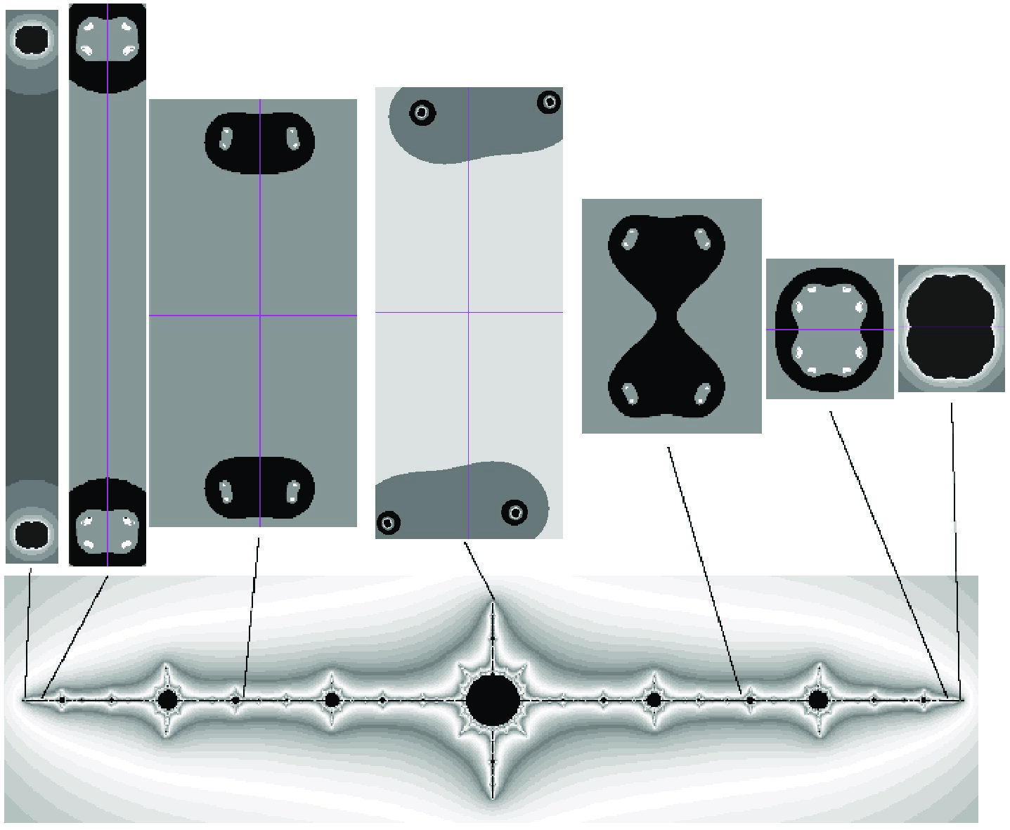 Figure 1
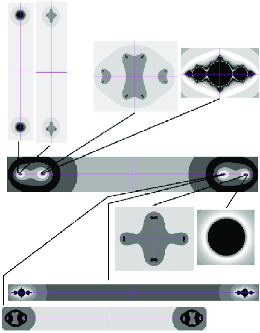 Figure 2
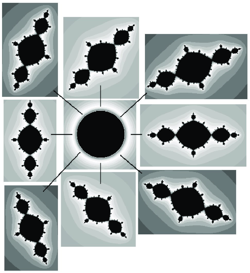 Figure 3
Peer Reviews
No public reviews on file for this paper yet. If you reviewed it on a platform where reviews are public (OpenReview, ICLR, NeurIPS, ICML), you can paste yours below so the community can read it here.
Videos
No videos yet. Explain this paper in a talk, walkthrough, or lecture? Add one.
Taxonomy
TopicsMathematical Dynamics and Fractals · Advanced Differential Equations and Dynamical Systems · Geometry and complex manifolds
Axiom A Polynomial skew products of
and their postcritical sets
Laura DeMarco1
Department of Mathematics
University of Chicago
5734 S. University Ave.
Chicago, IL 60637
USA
and
Suzanne Lynch Hruska2
Department of Mathematical Sciences
University of Wisconsin Milwaukee
PO Box 413
Milwaukee, WI 53201
USA
Abstract.
A polynomial skew product of is a map of the form , where and are polynomials, such that extends holomorphically to an endomorphism of of degree . For polynomial maps of , hyperbolicity is equivalent to the condition that the closure of the postcritical set is disjoint from the Julia set; further, critical points either iterate to an attracting cycle or infinity. For polynomial skew products, Jonsson ([Jon99]) established that is Axiom A if and only if the closure of the postcritical set is disjoint from the right analog of the Julia set. Here we present an analogous conclusion: critical orbits either escape to infinity or accumulate on an attracting set. In addition, we construct new examples of Axiom A maps demonstrating various postcritical behaviors.
11footnotetext: ,2Research supported in part by a grant from the National Science Foundation.
1. Introduction
A polynomial skew product of is a map , where and are polynomials. We will assume that is regular of degree , meaning that it extends holomorphically to an endomorphism of ; consequently the polynomials and both have degree .
In this paper, we study the postcritical set for Axiom A polynomial skew products, and we construct new examples of Axiom A maps demonstrating various postcritical behaviors. This is motivated by results in one-dimensional complex dynamics relating the behavior of the postcritical set to hyperbolicity.
For polynomial maps of , hyperbolicity is equivalent to the condition that the postcritical set is disjoint from the Julia set; by the classification of Fatou components, critical points are either in the basin of an attracting cycle or they escape to infinity under iteration (see e.g. [McM94, Theorem 3.13]). For polynomial skew products, Jonsson established that Axiom A is characterized by postcritical behavior [Jon99, Cor 8.3]: the postcritical set must be disjoint from the right analog of the Julia set. Here we present the analogous conclusion: critical points either escape to infinity or are in the basin of an attracting set.
Dynamics over . Let denote the Julia set of the base polynomial . We are primarily interested in the dynamics of restricted to . This invariant subset contains , the closure of the repelling cycles for , which coincides with the support of the measure of maximal entropy for [Jon99].
When is Axiom A, its nonwandering set is contained in , where is the finite set of attracting periodic points of . The dynamics of over reduces to one-dimensional complex dynamics, so the nontrivial part of the saddle set of is also contained in .
As preserves the family of vertical lines , the iterates form a composition of polynomial maps of of degree , with bounded coefficients for . The dynamics of such composition sequences have been studied in [FS91] and [Com06]. In our study of skew products in , we combine results about (hyperbolic) composition sequences with one- and two-dimensional complex iteration theory. We remark that Sumi also studies a notion of hyperbolicity for composition sequences in the setting of rational skew products [Sum01, Sum06].
Main result. If is Axiom A, let denote the union of the basic sets of saddle type in (see §2 for definitions). Its unstable manifold consists of all points for which there exists a backward orbit of converging to . Axiom A implies . Our main theorem shows that in , each of and plays the role of the one-dimensional attracting periodic orbits, in the following sense.
Set , and define the critical locus over by
[TABLE]
If is any subset of , its accumulation set111For a point , coincides with the -limit set of . is
[TABLE]
We will study the accumulation set as well as the pointwise and component-wise accumulation sets,
[TABLE]
where denotes the collection of connected components of . Each of these sets is closed, and we clearly have .
Theorem 1.1**.**
If is an Axiom A polynomial skew product of , then
[TABLE]
In particular, the first equality shows that each critical point in either tends to the saddle set or escapes to infinity. To explain the appearance of , we can compare to the invertible setting. The real, or smooth, -lemma states that if is a saddle periodic point, then the forward images of a disk transverse to which intersects a neighborhood of will tend to (see e.g. [Rob99, Chp. 5, Theorem 11.1]). In our setting, the critical locus (in fact any set transverse to and disjoint from ) is like such a disk (see Proposition 3.3).
Explicit families of Axiom A examples. Among dynamical systems with chaotic behavior, Axiom A maps are the most tractable. Jonsson has shown that the Axiom A maps form an open subset of the parameter space of all skew products, which allows him to define hyperbolic components as connected components of the subset of Axiom A maps ([Jon99, Corollary 8.15, Definition 8.16]).
In this paper, we construct examples of Axiom A maps supporting different chains of equalities or inequalities in Theorem 1.1, and distinguish the hyperbolic components of our examples. This work yields the next two results.
Proposition 1.2**.**
Polynomial skew products in the same hyperbolic component as a product have equality for every inclusion of Theorem 1.1.
Theorem 1.3**.**
There exist examples of Axiom A polynomial skew products , none of which are in the hyperbolic component of a product, such that:
- (1)
for , ; 2. (2)
for , ; 3. (3)
for , ; 4. (4)
for , .
Moreover, each is also Axiom A as an endomorphism from to itself.
There are few known examples of Axiom A endomorphisms in two (or more) dimensions. Fornaess and Sibony study examples of Axiom A endomorphisms of in [FS01, FS98]. Among polynomial skew products, Jonsson ([Jon99, §9]) lists known Axiom A maps to be: products of hyperbolic polynomial maps of , small perturbations of hyperbolic products, and he gives a degree 2 example of an Axiom A map not in the same hyperbolic component as any product. Diller and Jonsson ([DJ00]) generalize this last example for all . Their examples also satisfy (4) in Theorem 1.3. Sumi has communicated to the authors another new example of an Axiom A polynomial skew product satisfying (2) of Theorem 1.3, which is very different from ours. We describe his construction in Example 5.10.
Stability and holomorphic motions. One of our main tools for distinguishing hyperbolic components is holomorphic motions of . Jonsson established a general result about holomorphic motions of hyperbolic sets of holomorphic endomorphisms [Jon98, Theorem C], which implies that if is an Axiom A polynomial skew product, then moves holomorphically under perturbation. Further, we show:
Theorem 1.4**.**
For a holomorphic family of Axiom A polynomial skew products, the holomorphic motion of preserves the vertical fibration, inducing a holomorphic motion of each fiber Julia set .
A more precise statement is given in Theorem 4.2. As a corollary, if a polynomial skew product is in the same hyperbolic component as a product, then all fiber Julia sets are homeomorphic (Corollary 4.4). This answers a question from [Hru06], originally posed to the author by Eric Bedford. Our examples satisfying (1) and (2) of Theorem 1.3 will show that the converse is not true, for in those examples all fiber Julia sets are homeomorphic, but the maps are not in the same hyperbolic component as any product.
Theorem 1.4 also implies that the equalities and are preserved under perturbation (Propositions 5.4 and 6.3). We leave it as an open question to show that the equality is also preserved (see Question 8.2).
Organization of sections. In Section 2 we provide some needed prerequisite material on the dynamics of polynomial skew products, hyperbolic maps of , and general composition sequences of polynomials.
In Section 3, we prove Theorem 1.1.
In Section 4, we prove Theorem 1.4 on holomorphic motions.
In Section 5, we establish conditions giving equality for all inclusions in Theorem 1.1, prove Proposition 1.2, and provide specific examples of maps satisfying (1) and (2) of Theorem 1.3.
In Section 6, we establish a necessary and sufficient condition for in hyperbolic components (Lemma 6.4), and construct Axiom A skew products with base Julia set connected, but topologically varying fiber Julia sets (some connected, some disconnected). We show these maps satisfy (3) of Theorem 1.3. These maps are a perturbation of [Jon99, Example 9.7] (which is not Axiom A).
In Section 7, we produce Axiom A maps illustrating (4) of Theorem 1.3. These are a generalization of [DJ00, Example 3.9].
We close the paper with some open questions.
Acknowledgements
We thank Eric Bedford and Curt McMullen for helpful conversations during our work on this project, Greg Buzzard for feedback on drafts of the paper, Mattias Jonsson for pointing out Remark 5.9, Lois Kailhofer for providing insight on natural extensions and inverse limits, and Hiroki Sumi for describing Example 5.10. We would also like to thank the referee for his careful reading of the paper and many constructive suggestions.
2. Background
A polynomial map is a (regular) polynomial skew product if it has the form
[TABLE]
for polynomials and of degree , and if extends analytically as a map from to itself. We refer the reader to [Jon99] for a general treatment of polynomial skew products and proofs of many of the statements below.
Global dynamics. Fix a polynomial skew product . Let denote the filled Julia set of (the set of points with bounded orbit) and its Julia set. Let be the filled Julia set of . Set and in . The set
[TABLE]
is the closure of the repelling cycles of and also the support of its measure of maximal entropy. The nonwandering set of is the set of points having no neighborhood such that for all .
Vertical dynamics and expansion. For a fixed , we define , and set
[TABLE]
We have and . Let be the critical set of in .
Let be compact with (e.g. or is an attracting periodic point of ). Set
[TABLE]
and
[TABLE]
We say is vertically expanding over if there exist constants and such that
[TABLE]
for all , and all .
In this paper, we repeatedly use the following results.
Proposition 2.1**.**
[Jon99, Proposition 2.1]** For every polynomial skew product , is upper semi-continuous (in the Hausdorff topology), is lower semi-continuous, and the sequence of polynomials is normal exactly on .
Proposition 2.2**.**
[Jon99, Proposition 2.3]** For any , is connected if and only if for all .
Theorem 2.3**.**
[Jon99, Proposition 3.5]** If is vertically expanding over , then is continuous in the Hausdorff topology with . In particular, if is vertically expanding over , we have
[TABLE]
Theorem 2.4**.**
[Jon99, Theorem 3.1]** is vertically expanding over if and only if .
We do not define Axiom A in this paper, because we use only the following:
Theorem 2.5**.**
[Jon99, Theorem 8.2]** A polynomial skew product is Axiom A on if and only if
- (i)
* is expanding on (i.e. is hyperbolic);*
- (ii)
* is vertically expanding over ; and*
- (iii)
* is vertically expanding over .*
Moreover, if is Axiom A on , then the nonwandering set equals the closure of the set of periodic points of (equals the chain recurrent set).
Further, is Axiom A on if in addition,
- (iv)
the extension of to the line at infinity of is hyperbolic as a one-dimensional polynomial.
Hyperbolicity for endomorphisms of . For a non-invertible holomorphic mapping of , basic results and definitions for hyperbolicity and stability of an invariant set must be given in terms of the natural extension, , which is the space of all sequences of prehistories (backward orbits) in , with inducing which is a shift. See, for example, [Jon99, §A.2], [FS98, §2], and [DJ00, §1.1] for definitions and properties.
If is Axiom A, then its nonwandering set decomposes into a finite union of basic sets such that and is transitive on each . A basic set is of saddle type if its unstable (complex) dimension is 1.
For an Axiom A polynomial skew product, we let denote the union of basic saddle sets contained in . On these sets, is contracting in the fiber direction. Theorem 2.5 also yields that is the closure of the set of saddle periodic points with , since this theorem establishes that periodic points are dense in the nonwandering set.
The set is the subset of of unstable dimension 2.
The stable manifold of an invariant set is the set of all points for which the forward orbit converges to . The unstable manifold is the set of all points for which there exists a prehistory (backward orbit) , converging to , i.e., for all , and as .
In [Jon99, Corollary 8.14], Jonsson states that the natural extension of the nonwandering set of an Axiom A polynomial skew product is stable; i.e., if is a holomorphic map of which is -close to , then there is a homeomorphism conjugating to (and respects decomposition into basic sets), and can be chosen close to the identity. In fact, by [Jon98, Theorem B], moves holomorphically, in a sense which we will not define precisely. 222In this paper, the only stability result we use is that moves holomorphically for Axiom A polynomial skew products (see Section 4), but we state this alternate result for benefit of the reader.
General composition sequences of polynomial maps of . Fornaess and Sibony ([FS91]) study fundamental properties of Julia sets arising from compositions of sequences of arbitrarily chosen polynomial maps of , with uniformly bounded degrees and coefficients. Comerford ([Com06]) establishes an analog of the one-variable postcritical characterizations of hyperbolicity in this setting. We apply Comerford’s results to the composition of fiber maps along the orbit of a point . We state a key result here for our setting of skew products, though it was written for general composition sequences (with uniform bounds on degree and coefficients).
Theorem 2.6**.**
[Com06, Theorem 4.1]** Suppose is a polynomial skew product which is vertically expanding over . Let be a compact, connected subset of , for some . There exist and such that for all ,
[TABLE]
where diam# is the diameter in the spherical metric on . Further, depends only on , and in addition depends on the distance from to (in the spherical metric).
3. Saddle sets and the attractor of the postcritical set
Throughout this section, let be an Axiom A polynomial skew product of degree . Recall that denotes the union of the saddle basic sets in , and is the closure of the saddle periodic points with . In this section we prove Theorem 1.1.
Trapping radius. If , let denote the disk about of radius in the spherical metric on . For , the vertical neighborhood of of radius is the set
[TABLE]
The following lemma is a corollary of Theorem 2.6, and was observed by Comerford in the setting of general composition sequences.
Lemma 3.1**.**
Let be a closed subset of such that . Let denote the vertical neighborhood of of radius . Then there exists an and such that for all and , we have
[TABLE]
When the conclusion of Lemma 3.1 is satisfied, we say that is a trapping radius (for under ).
Proof.
Since is compact and is closed and disjoint from , there is an with , for all Thus, Theorem 2.6 applied to each connected component of the slice yields that there exists an such that for all and , we have
[TABLE]
since . ∎
Proposition 3.2**.**
The sets
[TABLE]
are disjoint from and have a trapping radius .
Proof.
First note that (since is a union of basic sets) and , so Lemma 3.1 clearly applies to . By Theorems 2.4 and 2.5, we have , and by definition,
[TABLE]
As accumulation sets always satisfy , Lemma 3.1 applies to each of these postcritical sets. ∎
The unstable manifold is an attractor. Recall the unstable manifold is the set of all points for which there exists a backward orbit converging to .
Proposition 3.3**.**
For any closed subset of , its accumulation set is contained in .
The following proof is adapted from [FS98], Propositions 4.2 and 4.5, where they prove an analogous result for “s-hyperbolic” endomorphisms of .
Proof.
Let be an open neighborhood of in on which is expanding. In particular, is strictly contained in . Fix . Its preimages must accumulate on the non-wandering set over , . Since , the existence of implies that the preimages will accumulate on .
Choose so that . By continuity, there exists a neighborhood of in so that . It follows that converges uniformly to as .
Fix a neighborhood of in and a radius . Then there is an integer so that is contained in for all . This in turn implies that lies in for all .
Finally, let be any closed subset of and its accumulation set. Choose the expanding neighborhood small enough so that . As and are arbitrary, we conclude that must be contained in . ∎
As an immediate corollary to Proposition 3.3, we obtain:
Corollary 3.4**.**
The accumulation set satisfies .
Points with bounded orbit. Let denote .
Lemma 3.5**.**
The unstable manifold satisfies
[TABLE]
Proof.
We clearly have the inclusion , because and . Fix . The the orbit of is bounded and its accumulation set must lie in the non-wandering set of . Proposition 3.3 implies that so is disjoint from , but then this implies that . Consequently is in the stable manifold . We have by [Jon99, Proposition A.4], so is in . ∎
Lemma 3.6**.**
.
Proof.
The inclusion is clear from the definitions. The converse follows from Proposition 3.3 and Lemma 3.5. ∎
Lemma 3.7**.**
We have .
Proof.
First note that the accumulation set of any point will be a subset of , or empty. Proposition 3.3 implies that , so Lemma 3.5 gives .
If is a period saddle point with , then . The polynomial is hyperbolic; hence its attracting periodic points, which are saddle points of , attract critical points in . Thus . Hence contains all saddle periodic points with . As is closed, it also contains the closure of all saddle periodic points over , which is . ∎
The immediate basin of a saddle set. The following proposition should be interpreted as an analog of the one-dimensional result, where there is always a critical point in the immediate basin of an attracting cycle. For any point , let denote the vertical Fatou component containing ; that is, the connected component of the vertical slice of containing .
Proposition 3.8**.**
There exists so that contains a critical point of for all .
We begin with a simple lemma about hyperbolic metrics on planar domains. Let denote a Euclidean disk with center and radius .
Lemma 3.9**.**
Suppose is a bounded domain with
[TABLE]
Then the hyperbolic metric of restricted to the disk is comparable to the Euclidean metric. Explicitly,
[TABLE]
for all .
Proof.
Recall that the hyperbolic metric on the unit disk (with constant curvature -1) is given by . The inclusions imply that
[TABLE]
Restricting to gives the desired estimate. ∎
Proof of Proposition 3.8. For each , let be the vertical Fatou component containing . These domains are uniformly bounded, since all are contained in . Choose so that for all . Let denote the hyperbolic distance function on the domain .
Let be a trapping radius for , as guaranteed by Proposition 3.2. Then for all , and for fixed , any , and all . Note that the spherical metric is comparable to the Euclidean metric on the bounded domain . In particular, for each with , Lemma 3.9 implies that
[TABLE]
when is sufficiently large. Consequently, the proper holomorphic map is strictly contracting in the hyperbolic metric for every . It follows that there exists a critical point of in for every . ∎
The above yields the following proposition, which will be useful for establishing .
Proposition 3.10**.**
For any , there is an such that
[TABLE]
Proof.
Let be the integer given in Proposition 3.8. Denote the critical locus of over by . The vertical expansion of implies that is uniformly bounded away from . As a critical set, note that contains no isolated points and is fiberwise continuous over (that is, is continuous). Recall that the saddle set is also uniformly bounded from and that is continuous over .
We can therefore construct a family of paths, one from each point in to a point in contained in the Fatou component , such that all paths are uniformly bounded from . Indeed, suppose to the contrary that there is a sequence of points in so that any path joining to in has distance to the boundary less than with . Pass to a subsequence so that in . Take any path in joining to . Then is some distance from the boundary of (and therefore from ). By the continuity of in and the continuity of , there are paths joining to in which remain distance from for all large . This contradicts the assumption.
Using Theorem 2.6, iterating forward by some iterates, the paths contract uniformly, implying that for each , there exists a point of in the Fatou component within spherical distance of . In other words, is contained in the vertical neighborhood about of radius . ∎
Equality of and the unstable manifold. Now we are ready to establish the final inclusion needed for the statement of Theorem 1.1.
Lemma 3.11**.**
We have .
Proof.
Let be a trapping radius for the postcritical set . Proposition 3.10 says that the set contains a vertical neighborhood of of some small radius. Since is continuous in the Hausdorff topology, continuity of guarantees that contains a neighborhood of in the ambient space .
Fix . Let be a prehistory tending to . Then is in for all sufficiently large . Let be the closest point to in the fiber . Because is a trapping radius, the image is very close to . Letting , we have . ∎
Proof of Theorem 1.1. The inclusions are clear from the definitions. Combine Lemma 3.7 with Corollary 3.4 and Lemma 3.11 to complete the proof. ∎
4. Stability and perturbations of products
In this section, we prove Theorem 4.2, showing that for holomorphic families of Axiom A skew products, the holomorphic motion of must preserve the vertical fibration. As an application, we see that if a polynomial skew product is in the same hyperbolic component as a product, then all fiber Julia sets are homeomorphic.
Holomorphic motions. Suppose is a subset of a complex manifold . As above, denotes a disk in centered at with radius . Then is a holomorphic motion of if is continuous and
- (1)
for all , 2. (2)
is holomorphic for each fixed , 3. (3)
is injective for each fixed .
Uniform expansion on . Let : be a holomorphic family of polynomial skew products of the form
[TABLE]
that is, each is a polynomial skew product of and the coefficients of and are holomorphic in . If is hyperbolic for each , and if each is vertically expanding over , we say that the family is uniformly expanding on . Note uniform expansion on is weaker than Axiom A.
Theorem 4.1**.**
[Jon98, Theorem C]** Let be a holomorphic family of polynomial skew products which is uniformly expanding on . Then there exists an and a holomorphic motion such that such that and
[TABLE]
on for all .
We show the holomorphic motion also preserves the vertical fibration:
Theorem 4.2**.**
Under the same hypothesis as in Theorem 4.1 we also have that is a skew product
[TABLE]
where
- (1)
* is a holomorphic motion of such that conjugates to , and* 2. (2)
for each , defines a holomorphic motion such that .
Proof.
Because the one-dimensional polynomials are hyperbolic, there exists a holomorphic motion conjugating to by the one-dimensional theory (see e.g. [McM94]). By the density of repelling cycles in , the motion is uniquely determined.
Let be a periodic point of , so is a periodic point of of the same period. Then the point must be a repelling periodic point of of constant period in . Consequently, for all . This holds for all periodic points of with , and by density of periodic points in the fiber Julia set , we obtain that the projection to the first coordinate of is for all . Finally, by the density of periodic points in , continuity of , and the fact that is continuous over , we obtain that for some function and all .
Since is a skew product, the motion therefore preserves the vertical fibration of the skew products . The proof of (2) then follows immediately from the properties of as a holomorphic motion. ∎
Perturbations of a product. Theorem 4.2 applied to a product gives the following.
Proposition 4.3**.**
Let be a holomorphic family of polynomial skew products which is uniformly expanding on . If is a product, then for each with , the fiber Julia sets are homeomorphic to for all .
Proof.
For the product , all fiber Julia sets are equal to . Let be the holomorphic motion guaranteed by Theorem 4.1. The result follows immediately from property (2) of Theorem 4.2. ∎
By Theorem 2.5, a product is Axiom A if and only if each of and are hyperbolic polynomial maps of . Thus for products, uniform expansion of is equivalent to Axiom A.
Corollary 4.4**.**
Suppose is an Axiom A polynomial skew product in the same hyperbolic component as a product . Then for all , the fiber Julia sets of are homeomorphic (to ).
Proof.
Because and are in the same hyperbolic component, they can be connected by a chain of holomorphic motions, as guaranteed by Theorem 4.1. By Proposition 4.3, the fiber Julia sets are homeomorphic to . ∎
In the following section, the family of examples will show that the converse to Corollary 4.4 is false. That is, the fiber Julia sets for these maps are all homeomorphic, but for appropriate choices of the parameter , they are not in the same hyperbolic component as a product.
5. Axiom A skew products with
In this section, we first provide some general conditions under which we have equality for all inclusions listed in Theorem 1.1 (Theorem 5.2). As a corollary, we see equality is preserved in hyperbolic components. We also show that equality holds for Axiom A products and their perturbations (Proposition 1.2). Finally, we give an infinite family of distinct, non-product Axiom A maps, for which equality holds:
Theorem 5.1**.**
Let and , for each . We have:
- (1)
* is Axiom A if and only if is hyperbolic.* 2. (2)
If is Axiom A, then it is in the same hyperbolic component as a product if and only if has an attracting fixed point. 3. (3)
If is Axiom A, then .
Criteria for . In this subsection, let be an Axiom A polynomial skew product. We now give necessary and sufficient conditions which guarantee equality for all inclusions in Theorem 1.1. As usual, if then , and we say is continuous if it is continuous in the Hausdorff topology. Recall is a Euclidean disk with center and radius .
Theorem 5.2**.**
The following are equivalent:
- (a)
; 2. (b)
* is continuous for all ;* 3. (c)
* is continuous for all .*
The implication (b) (a) was inspired by Robinson’s analogous statement for diffeomorphisms ([Rob99, Ch. 8, Theorem 6.2]).
Proof.
First we show that if then each of (a), (b), and (c) hold. Note (a) and (b) are satisfied vacuously. Now, implies that , which implies that by Lemma 3.6. Since (Theorem 2.3), this yields for all . Again applying Theorem 2.3, is continuous over for Axiom A, we conclude that (c) holds. Now assume that .
(a) (b): Suppose is not continuous over . Since is closed, we must have upper semi-continuity. Let be a point where lower semi-continuity fails. Then there is a sequence in and a so that for all . The local stable manifold of the point lies in in the vertical fiber, therefore the local unstable manifold (for any choice of prehistory) of must be transverse to the fiber (see e.g. [FS98, §2]). Thus for all near . This implies that .
(b) (c): Suppose is not continuous over . Again since is closed, we can assume that fails to be lower semi-continuous at a point . As is continuous, we must have , and there exists a sequence in so that .
By Lemma 3.6, . Let be a subsequence of iterates converging to a point as . By continuity of , for each fixed the images converge to as .
By continuity of , there is a neighborhood of in and a so that is disjoint from . Choose large enough so that lies ; then lies in for all sufficiently large. But , so the invariance of implies that . By shrinking , we obtain a sequence of points converging to such that , and we conclude that is not continuous.
(c) (a): By continuity of , and since is closed, there is a neighborhood of in such that .
Let be any point in . Then there is sequence of preimages with for all sufficiently large . This implies that . By complete invariance of , we obtain . Recalling that by Lemma 3.5, we conclude that . Therefore . ∎
Corollary 5.3**.**
If is connected for all , then .
Proof.
[Jon99, Lemma 3.7] states that if is vertically expanding over , and if for all , is connected, then is continuous. ∎
Stability under perturbations. We are now ready to prove Proposition 1.2, which states that Axiom A products and their perturbations satisfy . We first give a general proposition about perturbations.
Proposition 5.4**.**
Suppose and are in the same hyperbolic component. Then holds for if and only if it holds for .
Proof.
We apply the characterization of from Theorem 5.2. Suppose that is continuous for . By Theorems 4.1 and 4.2, there is a holomorphic motion of on a neighborhood of which restricts to a holomorphic motion of in every fiber over . By the Sullivan-Thurston -lemma ([ST86]), the motion of extends to a motion of the whole fiber , perhaps restricting the domain of the motion. Consequently, the topology of the filled Julia set is unchanged for nearby maps (i.e. the Fatou components move with ). The continuity of for then guarantees that we also have continuity of for .
Note that if is discontinuous for , then it must fail to be lower semi-continuous. Combining this with the continuity of , there exists a sequence in and a component of the interior of , so that for any fixed compact subset , is disjoint from for all large. The Sullivan-Thurston -lemma preserves this discontinuity under perturbation.
Finally, we can connect to by a finite chain of holomorphic motions which preserve the equality , proving the proposition. ∎
Proof of Proposition 1.2. Let be an Axiom A product. Then for all . From Theorem 5.2, it follows that for . Then Proposition 5.4 shows that all maps in same hyperbolic component as have . ∎
The family . We now give the proof of Theorem 5.1. Let , , and . For each , set
[TABLE]
From the definition of , we have
[TABLE]
Note that the critical locus of over is . Therefore,
[TABLE]
We begin with a lemma on the structure of .
Lemma 5.5**.**
For each , we have .
See Figure 1, which shows slices of for the map .
Proof.
First observe that the vertical derivative of along the curve is given by
[TABLE]
If is a repelling periodic point of of period , then the vertical derivative of along the orbit of satisfies . Thus the iterates of cannot be normal (in the fiber direction) along this orbit, so , by Proposition 2.1. Since is closed, for all .
Let . For the reverse inclusion, note that . By invariance, we have for all along the backward orbit . These points are dense in . By lower semi-continuity of (Proposition 2.1), we conclude that for all in . Therefore . ∎
Lemma 5.6**.**
* is Axiom A if and only if is hyperbolic.*
Proof.
Suppose is hyperbolic. Then the postcritical set for remains a bounded distance away from the Julia set . The description of for in Equation (2) and Lemma 5.5 imply that is therefore disjoint from . Consequently is vertically expanding over . Note that the attracting set for the base map is and for all . Therefore is also vertically expanding over , so is Axiom A.
Conversely, if is not hyperbolic, then the postcritical set of is not disjoint from . As coincides with , we conclude that is not disjoint from . Therefore is not vertically expanding over and thus not Axiom A. ∎
Lemma 5.7**.**
Suppose is Axiom A. Then is in the same hyperbolic component as a product if and only if has an attracting fixed point.
First, we recall some facts on the dynamics of the family (see e.g., [CG93, VIII.1]). The Mandelbrot set is
[TABLE]
For , the orbit of the critical point [math] escapes to infinity, is hyperbolic, and is a Cantor set. If is hyperbolic and in the interior of , then has an attracting cycle which attracts the orbit of the critical point [math].
Proof.
If lies in the same component as a product, then the product must be , because over the fixed point of in is given by the map (and by Theorem 4.2, the vertical fibration is preserved by holomorphic motions).
First suppose that has an attracting fixed point. Then is in the same hyperbolic component as (the main cardiod of the Mandelbrot set). Hence by Lemma 5.6, is in the same hyperbolic component as which in turn is in the same hyperbolic component as .
Now suppose is hyperbolic with . For the product we have . For the twisted map, Lemma 5.5 implies that , considered as a subset of . If and are in the same hyperbolic component, then we can connect and by a chain of holomorphic motions which preserve the vertical fibration (Theorem 4.2). These motions therefore induce an isotopy from to within the ambient space . But this is impossible because connected components of are circles which project to with degree 1, while connected components of are circles which project to with degree 2, and these are in different homotopy classes.
Alternatively, suppose is hyperbolic with an attracting cycle of period . Suppose that and are in the same hyperbolic component. Then by Theorem 4.2, and are conjugate on their Julia sets by a conjugacy which preserves fibers over . In particular, the conjugacy must be the identity over . Let (respectively ) be the subset of (resp. ) such that each slice (resp. ) is the boundary of the Fatou component in containing the critical point . This subset of is dynamically characterized in the following way: the slice (resp. ) is the smallest connected subset of which is mapped to its image with degree 2 by (resp. ). Therefore, the conjugacy must take to . Consequently, the conjugacy maps the image to . Note however that the fibers of these image sets over do not coincide: for the product we have a curve winding around whereas for we have two curves winding around and , contradicting the fact that the conjugacy is the identity over . ∎
Proof of Theorem 5.1. Combine Lemmas 5.6 and 5.7 for parts (1) and (2). When is not in the Mandelbrot set, the critical points escape so by Lemma 3.7 and we trivially obtain equality. For in a hyperbolic component in the Mandelbrot set, the map is connected, so part (3) for follows from Corollary 5.3. ∎
As a corollary, note by Proposition 5.4 that if is in the same hyperbolic component as any Axiom A , then for .
Remark 5.8**.**
By Theorem 2.5, since the extension of to the line at infinity is simply the map , we have is Axiom A on if and only if is Axiom A on .
Finally, suppose is Axiom A. Note that if has disconnected Julia set, then satisfies (1) of Theorem 1.3, while if lies in the Mandelbrot set, then satisfies (2) of Theorem 1.3.
Remark 5.9**.**
While the map does not lie in the same hyperbolic component of a product, it should be noted that it is semiconjugate to the product via the map . That is, , though this semiconjugacy does not extend regularly to . This was pointed out to the authors by Mattias Jonsson.
Sumi’s example. Sumi has communicated to the authors the following very interesting example of a nonproduct Axiom A polynomial skew product satisfying . In his example, is a Cantor set, and all fiber ’s are connected. He constructs similar examples in [Sum07].
Example 5.10**.**
For any and , let , , , and define by .
For appropriate choices of small, and large with even, the map
[TABLE]
is an Axiom A polynomial skew product of satisfying:
- (1)
; 2. (2)
; 3. (3)
* is a Jordan curve, but not a quasicircle, for a.e. , in the maximal entropy measure of ;* 4. (4)
* is not in the same hyperbolic component as any product.*
Sketch of Proof..
Axiom A and (1) can be proven by examining the postcritical set, in a similar way to our study of the family of maps found in Section 7.
By (1) and Proposition 2.2, we have is connected for every , so by Corollary 5.3 we get (2).
is contained in two disks, and , for a small (such that as ). The fiber maps for in are small perturbations of , and the fiber maps for in are small perturbations of . As a result, over the -fixed point of (in ) is a quasi-basillica (not a Jordan curve), and over the -fixed point of (in ) is a quasi-circle. Applying Lemmas 4.31 and 4.37 of [Sum07] then yields (3).
Finally, (4) follows from (3) and Corollary 4.4. ∎
6. Axiom A skew products with
In this section, we show that the equality is preserved in hyperbolic components (Proposition 6.3), and we construct an infinite family of Axiom A skew products in distinct hyperbolic components for which , yielding (3) of Theorem 1.3.
The -airplane. Let be the unique quadratic polynomial with periodic critical point of least period and real. For example, is the “airplane”. Then is a sequence of real numbers descending to , and the Julia set is connected for each . Let denote the -fixed point of , the point in with greatest real part.
Theorem 6.1**.**
Consider the sequence of skew products
[TABLE]
For all sufficiently large , is Axiom A and
- (1)
; 2. (2)
* consists of a single fixed point in the fiber ;* 3. (3)
* is disconnected for all , while is a quasicircle;* 4. (4)
* is connected;* 5. (5)
; 6. (6)
* is not in the same hyperbolic component as a product; and* 7. (7)
* is in the same hyperbolic component as if and only if .*
Each of the maps is a small perturbation of . Jonsson ([Jon99, Example 9.7]) shows is vertically expanding over , and has the same connectivity properties as (i.e., (3) and (4) of the theorem), but is not Axiom A since the base is not hyperbolic. Our examples are the first Axiom A examples with such connectivity properties, which turn out to be the key to constructing an example with . The outline of the proof of Theorem 6.1 is based on [Jon99, Example 9.7], but since is not contained in , our case is of increased complexity.
Remark 6.2**.**
Because is a small perturbation of , one might expect to be vertically expanding over because vertical expansion should be an open condition. For general composition sequences, hyperbolicity is open in the topology on the space of sequences [Com06, Corollary 3.2], but it is not open in the product topology, even with uniform coefficient bounds. Consider the sequence of sequences given by
[TABLE]
Then for each fixed , the composition sequence is not hyperbolic, because the critical point at is iterated towards the Julia set, the locus of non-normality (see [Com06, Theorem 1.3]). On the other hand, the sequence converges in the product topology to as , which is hyperbolic.
Small perturbations of skew products correspond to small perturbations of fiberwise compositions in the product topology (with uniform bounds on the coefficients), not the topology (unless the nearby maps are conjugate).
See Figure 2 for some slices of for a map of the type of Theorem 6.1.
Maps with .
Proposition 6.3**.**
Suppose and are in the same hyperbolic component. Then the equality holds for if and only if it holds for .
We reduce the proof to the following lemma.
Lemma 6.4**.**
If is Axiom A, then if and only if for any connected component of , we have either or .
Proof.
Suppose . Let be a connected component of . Since by Lemma 3.7, we also get . Thus is either empty or contained in . If , then . On the other hand, if , then since and is connected, by complete invariance of we must have .
Suppose for each connected component of , we have either or . If then . On the other hand, if , then combining complete invariance of with Proposition 3.3 and Lemma 3.5 yields . Thus , and the reverse inequality follows from the definitions. ∎
Proof of Proposition 6.3. Let . Suppose is a holomorphic family of polynomial skew products which are uniformly expanding on , with giving the map . Then by Theorems 4.1 and 4.2, there is an and a holomorphic motion which conjugates the dynamics and preserves the vertical fibration. In particular, induces one-dimensional holomorphic motions of and of the fiber Julia sets for each .
For sufficiently small and each , the critical points of are close to the critical points of . If a critical point of lies in , then the holomorphic motion of forces nearby points to lie in for all nearby . Similarly, a critical point in must remain in under perturbation.
Furthermore, the motion of ensures that connected components of are uniformly close to connected components of for all sufficiently small. Let be a connected component of . By Lemma 6.4, either or . Therefore, we have or for all connected components of for the maps .
Finally, connect to by a closed path in the hyperbolic component. This path can be covered by a finite collection of overlapping open sets, on which the relation of to connected components of as described above is constant. The main result then follows from Lemma 6.4. ∎
The remainder of the section is devoted to the Proof of Theorem 6.1.
Proof of Theorem 6.1. Let where is the -airplane defined at the beginning of the section. Our most difficult task in this proof will be to establish that is Axiom A for sufficiently large. Since is a hyperbolic polynomial, by Theorem 2.5, we need only show is vertically expanding over and . To check vertical expansion we will apply Theorem 2.4, and show the postcritical set over is disjoint from the fiber Julia sets.
Hence, our first step is to provide two lemmas, locating first (in Lemma 6.5) the base filled Julia set (which contains both and ), and then (in Lemma 6.6) the fiber ’s for . As usual, we let denote the open disk in centered at with radius . For , we denote a closed rectangle around by
[TABLE]
and let .
Lemma 6.5**.**
There is a sequence such that .
Proof.
Let be the escape-rate function of . Then is continuous as a function of both and (see e.g. [CG93, VIII: Theorem 3.3]. As a consequence, the mapping is lower semi-continuous (because ), while is upper semi-continuous (because ). Hence for , we have . Thus is continuous at .
Note also that the logarithmic capacity of is 1 for all (see e.g. [CG93, VIII: Theorem 3.1]). Since is in the Mandelbrot set, , because any connected set of logarithmic capacity 1 has diameter bounded by 4, and is symmetric about the origin. Thus there is a sequence such that . ∎
Recall that the fiber map is independent of .
Lemma 6.6**.**
There is an such that for all and all , we have
- (i)
, and 2. (ii)
.
Proof.
By Lemma 6.5, there is an such that if . Then for and , we have , proving (i). In particular, , so the point escapes to infinity, proving (ii). ∎
Now we can easily show vertical expansion over .
Lemma 6.7**.**
* is vertically expanding over the attracting cycle of .*
Proof.
Note that is real, and note . Let . We show escapes. Let . Then for some , we have . But then , since is real. Hence by Lemma 6.6, , so for all . Thus is vertically expanding over . ∎
Establishing vertical expansion over is the work of the next couple of pages. Here is an overview. Note . We follow the outline of [Jon99, Example 9.7]. Fix a small , setting suffices for our proof. The idea is that first, if and , then a small neighborhood of the real axis in the fiber immediately escapes (which contains by Lemma 6.6). Next, if and , then the orbit under marches into ; further, for fixed , there is a uniformity in the number of iterates it takes for the orbit of any to land in , for all sufficiently large (Lemma 6.8). Combining the previous two ideas yields that critical orbits over escape and uniformly avoid (Lemma 6.9). Then in fibers over , we show a small neighborhood of the origin is mapped into itself (Lemma 6.10). Hence critical points over remain near the origin (and in ) as long as remains in , then once lands outside of , the previous case shows the orbits escape (Lemma 6.11 (i)). We add to this the dynamics of in the -fiber (Lemma 6.11 (ii)), to show the critical orbits in avoid (Lemma 6.11 (iii)). Finally, we combine the above to get critical orbits over are uniformly bounded away from for sufficiently large (Lemma 6.12).
The following two lemmas locate the postcritical set in . We first make a statement about the dynamics in the base (Lemma 6.8), then apply to the fibers (Lemma 6.9). Let be chosen as in Lemma 6.6.
Lemma 6.8**.**
There exist and such for all and , there is a with .
Proof.
Let be the external ray landing map for . Since is hyperbolic, is well-defined and continuous, and it semi-conjugates on with angle doubling on . Recall that is the -fixed point of .
First, we show that for any , there is a and so that
[TABLE]
for all
As in the proof of Lemma 6.5, the continuity of the escape-rate function in both and implies that the harmonic measure for the filled Julia set of is weakly continuous in . Furthermore, the measure coincides with the push-forward of Lebesgue measure on by the external ray landing map.
Fix and consider . Let be a bump function supported in with on the box . Then
[TABLE]
for some . This implies that at least of the total angle lands in . By continuity of the landing map for and the symmetry of , we have that contains the interval .
By weak continuity, the integral varies continuously in . Therefore
[TABLE]
for all sufficiently large . For these , the total angle landing in is bounded below by , and because is real, we have maintained the symmetry of . Therefore, contains the interval for all sufficiently large. Setting yields (3).
Finally, because the landing map defines a semiconjugacy between angle doubling on and on , there exists a uniform so that the finite orbit contains an element with for all and all . ∎
For given skew product , let denote the composition of fiber maps (recall the fiber map is independent of ). Recall by Lemma 6.6, we know for .
Lemma 6.9**.**
Let be given by Lemma 6.8. There exist and so that
[TABLE]
for all and .
Proof.
By Lemma 6.5, there exists so that
[TABLE]
for all . Choose with .
Fix and . Let denote the orbit of . Fix with and let .
Let be the least integer such that . If for some , then we conclude by Lemma 6.6 that for all , hence . Thus, we may assume that for all .
From the formula for , we have that , so that . By induction we obtain
[TABLE]
with the final inequality by our choices of and . Thus,
[TABLE]
We conclude that , so by Lemma 6.6. ∎
Next, we analyze the postcritical set over .
Lemma 6.10**.**
For any , there exists so that for all and , is contained in the interior of .
Proof.
Fix . By Lemma 6.5, we may choose so that for all .
Fix , , and , and let . Then
[TABLE]
and
[TABLE]
because . ∎
Let and be given by Lemma 6.9, and let be given by Lemma 6.10. We may assume and .
Lemma 6.11**.**
For all , we have
- (i)
* for all , and*
- (ii)
; hence
- (iii)
**
Proof.
First note that any point leaves after some number of iterates of . Therefore, (i) follows immediately from Lemmas 6.10, 6.9, and 6.6. Statement (ii) follows because , and Lemma 6.10 shows that the iterates of form a normal family on , hence by Proposition 2.1. Recalling that , (i) and (ii) yield (iii). ∎
Finally, we show how to combine the above to show the critical orbits over avoid , giving us vertical expansion over .
Lemma 6.12**.**
For all , is vertically expanding over .
Proof.
We analyze the postcritical set of . For , let .
For the case , the orbit lies in for all , by Lemma 6.10. By Lemma 6.11 (iii), the orbit is uniformly bounded away from .
For , let be the least integer such that . By Lemma 6.10, we have in the interior of for all , so by Lemma 6.11 (iii), lies a definite distance away from . Complete invariance of (and ) and the uniform in the statement of Lemma 6.9 implies that all for are uniformly bounded away from (and ), since (Lemma 6.6). The previous sentence also applies to critical points when . ∎
That is Axiom A for sufficiently large follows from the fact that is hyperbolic, Lemmas 6.7 and 6.12, and Theorems 2.4 and 2.5.
Finally, we turn to statements (1)–(7) of the theorem. Lemma 6.11 shows that all critical points except the one in the fiber over escape, and it is clear from the construction that is attracted to a fixed point in its fiber. Recalling that from Lemma 3.7, we find that is precisely this fixed point.
Because the critical points escape for , the Julia sets are disconnected for (Proposition 2.2), while is a quasicircle because is a small perturbation of . As the base is connected, it follows that is connected [Jon99, Lemma 6.7].
Next, since is connected, is a single connected component. Hence . But we showed the critical point is bounded, while the rest escape. Hence Lemma 6.4 yields .
Proposition 6.3 says the equality is preserved in hyperbolic components, and we know equality holds for products (Proposition 1.2); therefore, is not in the same hyperbolic component as a product.
Finally, and are in distinct hyperbolic components for , because and are in distinct hyperbolic components, and holomorphic motions of induce motions of the base by Theorem 4.2. ∎
Remark 6.13**.**
A map from Theorem 6.1 which is Axiom A in extends to the line at infinity as the map , hence is also Axiom A on . Such a map satisfies (3) of Theorem 1.3.
7. Axiom A skew products with
In this section, we construct an infinite family of Axiom A skew products in distinct hyperbolic components which satisfy , giving (4) of Theorem 1.3.
Theorem 7.1**.**
Given any two hyperbolic, monic polynomials of degree , and positive integers , there exists an Axiom A polynomial skew product such that
- (1)
* is a Cantor set, with two disjoint, forward-invariant compact subsets and such that is conjugate to the one-sided full shift on symbols;* 2. (2)
, thus is disconnected if ; 3. (3)
for each , the restriction is a small perturbation of the product ; 4. (4)
, where and if and only if not all critical points of escape; and 5. (5)
if for either or , then and the hyperbolic component containing does not contain a product.
Our construction is inspired by Proposition 3.8 and Example 3.9 of [DJ00], where the authors provide examples of polynomial skew products which are Axiom A on and have “nonterminal” (not minimal) basic saddle sets (so therefore are not in the same hyperbolic component as any product). Their fiber maps are derived from a combination of and for a large .
In our generalization, if has an attracting cycle , then will have a (nonminimal) saddle basic set over with of topological entropy (compare [DJ00, Proposition 3.8]). From the construction, we will see that the saddle set for is precisely the union of the saddle basic sets over all attracting cycles of and .
Figure 3 shows slices of for a map with .
Proof of Theorem 7.1. For clarity of exposition, we begin with a detailed construction for the case where . Hence, fix a hyperbolic, monic polynomial of degree , and positive integers .
First we define a base polynomial , for any (the constants and will be chosen later based on ). Fix distinct points in and in . Let . Set with chosen so that is a disjoint union of disks, compactly contained in , each univalently mapped by onto . For , define
[TABLE]
Then is a forward-invariant subset of , and is a Cantor set if or a single point if . In fact, is isomorphic to the full one-sided shift on symbols. Note in the case that and are the two fixed points of . Finally, since we see and are disjoint. Hence for any choice of , the map satisfies (1) of the theorem. Note also that is hyperbolic with no attracting cycles.
Define a norm on the space of polynomials of degree as the maximum of the absolute values of the coefficients. Choose small so that if is any sequence of polynomials with for all , then the composition sequence is hyperbolic with a uniform postcritical distance to the sequence Julia sets (see [Com06, Corollary 3.2]). In particular, the Julia set for the composition sequence will be a small perturbation of .
Lemma 7.2**.**
There exist and so that
- (i)
,
- (ii)
* for all with ,*
- (iii)
, and
- (iv)
for any sequence with for all , the critical points of and their images under the composition sequence are uniformly bounded away from the annulus and the union of its preimages, .
Proof.
Properties (i), (ii), and (iii) can clearly be satisfied by choosing large enough and small. Properties (i) and (ii) imply that the filled Julia set of is contained in the disk . Therefore, property (iv) is only relevant if has escaping critical points, because is hyperbolic and accumulates on the Julia set . Let
[TABLE]
be the escape-rate function for . By selecting large enough, the images of the critical points of under iterates of can be arranged to be disjoint from because the modulus is independent of , while a fundamental annulus has modulus as . It follows that the postcritical set of is uniformly bounded away from . Property (iv) holds for nearby sequences by continuity. ∎
Set
[TABLE]
and let . For our skew product map, we define
[TABLE]
Lemma 7.3**.**
The fiber filled Julia sets for satisfy
[TABLE]
Proof.
From the definition of and the choice of and in Lemma 7.2, we have that and implies:
[TABLE]
and for , the inequality implies:
[TABLE]
Therefore these points escape to infinity under iteration of .
For , the sequence of polynomials satisfies for all ; by the choice of , properties (i) and (ii) of Lemma 7.2 imply that . ∎
For , the composition sequences are hyperbolic by our choice of with uniform postcritical distance [Com06, Theorem 1.3], so is vertically expanding over .
The critical points of over coincide with the critical points of . For , let . There is a smallest integer so that and (with ). From (iv) of Lemma 7.2, the images of the critical points remain in for all . Furthermore, by Lemma 7.3. Let . From Lemma 7.2, the postcritical set of any sequence with for all is uniformly bounded away from . By invariance of the filled Julia sets, the postcritical points are therefore uniformly bounded away from the filled Julia set for all . For , we have , so these points are also uniformly bounded away from .
We conclude that is vertically expanding over all of . Since has no attracting periodic points, is Axiom A by Theorem 2.5. Note that all critical points over escape. Combining this with Proposition 2.2 yields (2) of the theorem.
In the case of distinct and , each monic, hyperbolic polynomials of degree , choose and as in Lemma 7.2 to work for both and , set and . Write
[TABLE]
[TABLE]
where for . Set
[TABLE]
and
[TABLE]
Then the arguments above show that is vertically expanding over (hence Axiom A), and that (1) and (2) hold, and further, behaves as a small perturbation of the product over and as a small perturbation of over , which establishes (3) of the theorem.
For (4) of the theorem, first recall that (Lemma 3.7), and note , since we showed above that all critical points over escape. Since and are disjoint and each is forward invariant, we conclude with , and any basic set in is contained in one of or . Note also is the closure of the saddle periodic points of in .
Let be any periodic point of in , say of period (at least one exists since is the full one-sided shift on symbols). Then by (3), is a small perturbation of , so its attracting cycles are perturbations of those for . Thus the saddle basic sets of in are in one-to-one correspondence with attracting periodic points of . Hence precisely when has an attracting cycle, which, since is hyperbolic, is equivalent to having a critical point which does not escape.
To show (5) of the theorem, assume that has an attracting cycle . Then as above, has an associated saddle basic set over . Let be a critical point of such that as .
Fix and let be a sequence of preimages such that for all . By the construction of (in particular, the choice of ), the point lies in a small neighborhood of in for all sufficiently large. Therefore this neighborhood contains a point in the accumulation set . Consequently, for all , we have
[TABLE]
On the other hand, because the connected components of are points, while by Lemma 3.7. As , we conclude that .
Finally, recall that products must have equality of by Proposition 1.2, and this equality is preserved in hyperbolic components (Proposition 5.4). Therefore, in the case that , we can conclude that is not in the same hyperbolic component as a product. This concludes the proof of Theorem 7.1. ∎
Remark 7.4**.**
The extension of an Axiom A (as constructed in Theorem 7.1) to the line at infinity is , where was chosen in defining at the beginning of the proof, and is very large (so that has a Cantor Julia set). Thus is expanding on the Cantor Julia set on the line at infinity, so is Axiom A on . Thus satisfies (4) of Theorem 1.3.
8. Remaining Questions
Question 8.1**.**
In our examples, we focused on maps of degree two. In higher degree, more varied phenomena than we discussed might occur.
Let be an Axiom A polynomial skew product of degree . In the space of polynomial maps of of degree , let be the hyperbolic polynomials with Cantor Julia set and be the hyperbolic polynomials with connected Julia set. If , then , and if , then . All hyperbolic polynomials of degree two are either in or . But in higher degree this is not the case.
Thus we ask: do there exist Axiom A polynomial skew products such that and:
- (1)
for ; 2. (2)
for ; 3. (3)
for ?
Question 8.2**.**
Does there exist a characterization of the equality in a similar spirit to Lemma 6.4 or Theorem 5.2? And is this equality preserved in hyperbolic components?
Propositions 5.4 and 6.3 imply that (1) of Question 8.1 is preserved in hyperbolic components. We are asking if the same is true for (2) and (3).
Question 8.3**.**
Nekrashevych [Nek05] shows that the rational skew product of given by
[TABLE]
is Axiom A, with connected base Julia set, and all fiber Julia sets connected, but such that not all fibers are homeomorphic (for example, over the fixed points of the base map, one fiber map is the rabbit, while another one is the airplane). This suggests there is no dynamical obstruction to a polynomial skew product of which is fully connected yet with varying fiber dynamics, but no such example has been exhibited.
By Corollary 4.4, such a map would not be in the same hyperbolic component as any product, and by Corollary 5.3, it would satisfy .
The reference list from the paper itself. Each links out to its DOI / PubMed record.
- 1[CG 93] Lennart Carleson and Theodore W. Gamelin. Complex dynamics . Universitext: Tracts in Mathematics. Springer-Verlag, New York, 1993.
- 2[Com 06] Mark Comerford. Hyperbolic non-autonomous Julia sets. Ergodic Theory Dynam. Systems , 26(2):353–377, 2006.
- 3[DJ 00] Jeffrey Diller and Mattias Jonsson. Topological entropy on saddle sets in 𝐏 2 superscript 𝐏 2 {\bf P}^{2} . Duke Math. J. , 103(2):261–278, 2000.
- 4[FS 91] John Erik Fornæss and Nessim Sibony. Random iterations of rational functions. Ergodic Theory Dynam. Systems , 11(4):687–708, 1991.
- 5[FS 98] J.E. Fornæss and N. Sibony. Hyperbolic maps on 𝐏 2 superscript 𝐏 2 \mathbf{P}^{2} . Math. Ann. , 311(2):305–333, 1998.
- 6[FS 01] John Erik Fornæss and Nessim Sibony. Dynamics of 𝐏 2 superscript 𝐏 2 {\bf P}^{2} (examples). In Laminations and foliations in dynamics, geometry and topology (Stony Brook, NY, 1998) , volume 269 of Contemp. Math. , pages 47–85. Amer. Math. Soc., Providence, RI, 2001.
- 7[Hru 06] S.L. Hruska. Rigorous numerical studies of the dynamics of polynomial skew products of ℂ 2 superscript ℂ 2 \mathbb{C}^{2} . In R. Devaney and L. Keen, editors, Complex Dynamics , volume 396 of Contemporary Mathematics , page 208, Providence, RI, 2006. American Mathematical Society. Proceedings of an AMS-IMS-Siam Joint Summer Research Conference on Complex Dynamics, June 13–17, 2004.
- 8[Jon 98] Mattias Jonsson. Holomorphic motions of hyperbolic sets. Michigan Math. J. , 45(2):409–415, 1998.