Interactions, superconducting $T_c$, and fluctuation magnetization for two coupled dots in the crossover between the Gaussian Orthogonal and Unitary ensembles
Oleksandr Zelyak, Ganpathy Murthy, Igor Rozhkov

TL;DR
This paper analyzes the effects of crossover regimes between Gaussian Orthogonal and Unitary ensembles on two coupled quantum dots, revealing nonmonotonic behavior of critical temperature and fluctuation magnetization influenced by magnetic flux.
Contribution
It introduces a diagrammatic approach to describe Green's functions in crossover regimes and investigates the impact on superconducting transition and magnetization in coupled quantum dots.
Findings
Critical temperature exhibits nonmonotonic dependence on magnetic flux.
Fluctuation magnetization can be diamagnetic or paramagnetic.
Separate scaling functions describe diffuson and cooperon contributions.
Abstract
We study a system of two quantum dots connected by a hopping bridge. Both the dots and connecting region are assumed to be in universal crossover regimes between Gaussian Orthogonal and Unitary ensembles. Using a diagrammatic approach appropriate for energy separations much larger than the level spacing we obtain the ensemble-averaged one- and two-particle Green's functions. It turns out that the diffuson and cooperon parts of the two-particle Green's function can be described by separate scaling functions. We then use this information to investigate a model interacting system in which one dot has an attractive s-wave reduced Bardeen-Cooper-Schrieffer interaction, while the other is noninteracting but subject to an orbital magnetic field. We find that the critical temperature is {\it nonmonotonic} in the flux through the second dot in a certain regime of interdot coupling. Likewise, the…
Click any figure to enlarge with its caption.
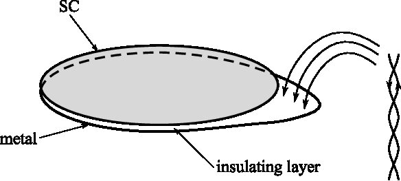 Figure 1
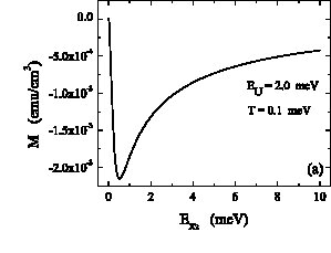 Figure 1
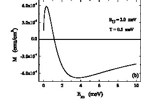 Figure 1
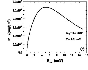 Figure 1
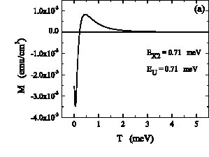 Figure 1
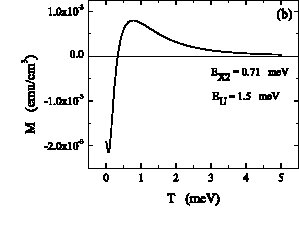 Figure 1
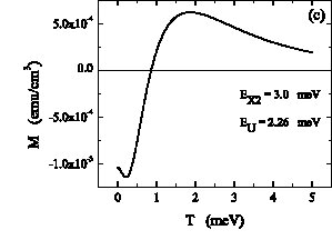 Figure 1
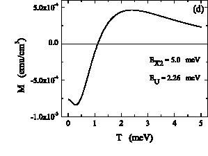 Figure 1
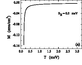 Figure 1
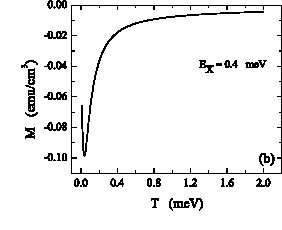 Figure 1
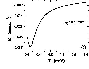 Figure 1
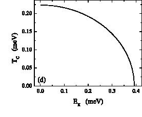 Figure 1
 Figure 1
 Figure 2
 Figure 3
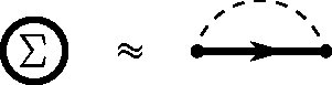 Figure 4
 Figure 5
 Figure 7
 Figure 8
 Figure 9
 Figure 10
 Figure 11
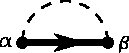 Figure 12
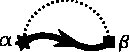 Figure 13
 Figure 14
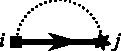 Figure 15
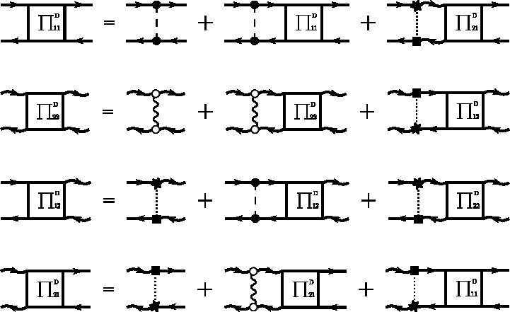 Figure 18
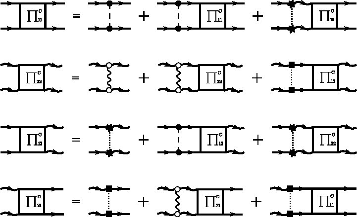 Figure 19
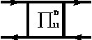 Figure 21
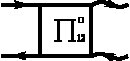 Figure 22
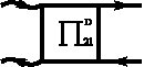 Figure 23
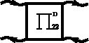 Figure 24
 Figure 25
 Figure 26
 Figure 27
 Figure 29
 Figure 29
 Figure 30
 Figure 31
 Figure 31
Peer Reviews
No public reviews on file for this paper yet. If you reviewed it on a platform where reviews are public (OpenReview, ICLR, NeurIPS, ICML), you can paste yours below so the community can read it here.
Videos
No videos yet. Explain this paper in a talk, walkthrough, or lecture? Add one.
Interactions, superconducting , and fluctuation
magnetization for two coupled dots in the crossover between the Gaussian Orthogonal and Unitary ensembles
Oleksandr Zelyak
Ganpathy Murthy
Department of Physics and Astronomy, University of Kentucky, Lexington, Kentucky 40506, USA
Igor Rozhkov
Department of Physics, University of Dayton, 300 College Park, Dayton, OH 45469
Abstract
We study a system of two quantum dots connected by a hopping bridge. Both the dots and connecting region are assumed to be in universal crossover regimes between Gaussian Orthogonal and Unitary ensembles. Using a diagrammatic approach appropriate for energy separations much larger than the level spacing we obtain the ensemble-averaged one- and two-particle Green’s functions. It turns out that the diffuson and cooperon parts of the two-particle Green’s function can be described by separate scaling functions. We then use this information to investigate a model interacting system in which one dot has an attractive -wave reduced Bardeen-Cooper-Schrieffer interaction, while the other is noninteracting but subject to an orbital magnetic field. We find that the critical temperature is nonmonotonic in the flux through the second dot in a certain regime of interdot coupling. Likewise, the fluctuation magnetization above the critical temperature is also nonmonotonic in this regime, can be either diamagnetic or paramagnetic, and can be deduced from the cooperon scaling function.
quantum dot, scaling function, crossover, quantum criticality
pacs:
73.21.La, 05.40.-a, 73.50.Jt
I Introduction
The idea of describing a physical system by a random matrix Hamiltonian to explain its spectral properties goes back to WignerWigner (1955, 1957). It was further developed by Dyson, Mehta and others, and became the basis for Random Matrix Theory (RMT)Mehta (2004). First introduced in nuclear physics, RMT has been used with great success in other branches of physics and mathematics. A notable example was a conjecture by Gorkov and EliashbergGorkov and Eliashberg (1965) that the single-particle spectrum of a diffusive metallic grain is controlled by RMT. This conjecture was proved by Altshuler and ShklovskiiAl’tshuler and Shklovskii (1986) who used diagrammatic methods and by Efetov who used the supersymmetry methodEfetov (1983). In 1984 Bohigas, Giannoni and SchmitBohigas et al. (1984) conjectured that RMT could also be employed in the study of ballistic quantum systems whose dynamics is chaotic in the classical limit. Their conjecture broadened the area of applicability of RMT enormously and was supported by numerous ensuing experiments and numerical simulations Bohigas et al. (1984); Hönig and Wintgen (1989); Zimmermann et al. (1988); Deus et al. (1995). The crucial energy scale for the applicability of RMT is the Thouless energy , where is the time for a wave packet to spread over the entire system. For a diffusive system of size , we have , while for a ballistic/chaotic system we have , where is the Fermi velocity.
In this paper we consider a system of two quantum dots/nanoparticles which are coupled by a hopping bridge. The motion of electrons inside each dot can be either ballistic or diffusive. In the case of ballistic dots we assume that the dots have irregular shapes leading to classically chaotic motion, so that RMT is applicable.
RMT Hamiltonians fall into three main ensemblesMehta (2004). These are the Gaussian Orthogonal Ensemble (GOE), Gaussian Unitary Ensemble (GUE), and Gaussian Symplectic Ensemble (GSE). They are classified according to their properties time-reversal (TR). The Hamiltonians invariant with respect to TR belong to the GOE. An example of GOE is a quantum dot which has no spin-orbit coupling and is not subject to an external magnetic field. GUE Hamiltonians, on the contrary, are not invariant with respect to TR and describe motion in an orbital magnetic field, with or without spin-orbit coupling. Hamiltonians from GSE group describe systems of particles with Kramers degeneracy that are TR invariant but have no spatial symmetries, and correspond to systems with spin-orbit coupling but with no orbital magnetic flux. In our paper we only deal with the first two classes.
For weak magnetic flux the spectral properties of the system deviate from those predicted by either the GOE or the GUE Sommers and Iida (1994). In such cases the system is said to be in a crossoverMehta (2004). For these systems the Hamiltonian can be decomposed into real symmetric and real antisymmetric matrices:
[TABLE]
where is the crossover parameterAleiner et al. (2002) which is equal, up to factors of order unity, to , where is the magnetic flux through the dot, and is the quantum unit of magnetic flux. Note that the gaussian orthogonal and unitary ensembles are limiting cases of and respectively.
To understand the meaning of the crossover parameter consider the Aharonov-Bohm phase shift picked up by a ballistic electron in a single orbit in the dot:
[TABLE]
For one turn the flux enclosed by the trajectory is proportional to , where is the size of the dot. After turns the total flux is , where factor originates from the fact that electron has equal probability to make clockwise or counterclockwise orbits, and thus does a random walk in the total flux enclosed. The minimal phase shift for the electron to notice the presence of the magnetic flux is of the order , and thus the minimal cumulative flux enclosed by the orbit should be . This leads to , while the time to make turns is (for a ballistic/chaotic dot). From the Heisenberg uncertainty principle the associated energy scale is:
[TABLE]
where is the ballistic Thouless energy Altland et al. (1996). For a diffusive dot it should be substituted by the diffusive Thouless energy . One can see that when is equal to , is equal to which means that energy levels are fully crossed over.
In this paper the reader will encounter many crossover parameters, and thus many crossover energy scales. By a line of argument similar to that leading to Eq. (3), it can be shown that to every crossover parameter there is a corresponding energy scale .
Breaking the time reversal symmetry of system changes the two-particle Green’s function. While the two-particle Green’s function can in general depend separately on , , and the measurement frequency , it turns out that in the universal limit , it becomes a universal scaling function of the ratio . The scaling function describes the modification of as one moves away from the “critical” point . The limits of the scaling function can be understood as follows: If the measurement frequency is large (small) compared to the crossover energy scale , the takes the form of the GOE (GUE) ensemble correlation function. If , the Green’s function describes the system in crossover regime.
The one-particle Green’s function is not critical as , although it gets modified by the interdot coupling. The two-particle Green’s function always has a diffuson mode Efetov (1999), that diverges for small in our large- approximation, which means that our results are valid on scales much larger than mean level spacing. This divergence is not physical and will be cut off by vanishing level correlations for in a more exact calculationAbrikosov (1975). On the other hand, the energy scale should be smaller than Thouless energy of the system for RMT to be applicable. These limitations hold for the crossover energy as well. In what follows we study the regime corresponding to .
The other term that appears in the two-particle Green’s function is a cooperon mode. In general the cooperon term is gapped if at least one of the crossover parameters is different from zero. In the case when the total Hamiltonian of the system is time reversal invariant, all the crossover parameters are zero and the cooperon, just like the diffuson, becomes gapless. Finally, when each part of compound system belongs to the GUE (the case when all crossover parameters are much larger than ) the cooperon term disappears.
Our study has a two-fold motivation. The first part comes from works on coupled structures with noninteracting particles in acoustic and electronic systemsWaugh et al. (1995); Weaver and Lobkis (2000); Tschersich and Efetov (2000), and crossovers Fal’ko and Efetov (1994); J. B. French and Tomsovic (1988); van Langen et al. (1997); Pandey and Mehta (1983); Sommers and Iida (1994). We focus on a complete description of the crossover regimes in all three regions (the two dots and the bridge) and define scaling functions for the diffuson and cooperon parts of the two-particle Green’s function. Using parameters analogous to we describe crossover regimes in dots 1 and 2 and the effects of the tunable hopping between them. Varying these parameters allows us to obtain results for various physical realizations, when different parts of the compound system behave as pure GOE, GUE, or belong to the crossover ensemble. In electronic systems it is easy to break time-reversal by turning on an external orbital magnetic flux. In acoustic systems one can break time-reversal by rotating the system or a part thereof. As mentioned before, the system of two dots coupled by hopping has been investigated before using supersymmetry methodsTschersich and Efetov (2000). However, the authors considered only the GUE, whereas here we are interested in the full crossover. In fact, the crossover is essential to the second aspect of our work, as will become clear immediately.
The second part of our motivation is the possibility of using the information gained in noninteracting systems to predict the behavior of interacting systemsAdam et al. (2002, 2003); Alhassid and Rupp (2003); Murthy (2004). We consider interacting systems controlled by the Universal HamiltonianAndreev and Kamenev (1998); Brouwer et al. (1999); Baranger et al. (2000); Kurland et al. (2000), which is known to be the interacting low-energy effective theoryMurthy and Mathur (2002); Murthy and Shankar (2003); Murthy et al. (2004) deep within the Thouless band in the renormalization groupShankar (1994, 1991) sense for weak-coupling when the kinetic energy is described by RMT and the Thouless number . For the GOE the Universal Hamiltonian has the formAndreev and Kamenev (1998); Brouwer et al. (1999); Baranger et al. (2000); Kurland et al. (2000)
[TABLE]
where is the total particle number, is the total spin, and . In addition to the charging energy, has a Stoner exchange energy and a reduced superconducting coupling . This last term is absent in the GUE, while the exchange term disappears in the GSE.
In this paper we concentrate on the reduced Bardeen-Cooper-Schrieffer (BCS) coupling which leads to a mean-field superconducting state when . Previous work by one of usMurthy (2004) sets the context for our investigation. We consider an interacting system which has a single-particle symmetry and a quantum phase transition in the limit . An example relevant to us is a superconducting nanoparticle originally in the GOE. It has the reduced BCS interaction and time-reversal symmetry, and the (mean-field) quantum phase transition is between the normal and superconducting states and occurs at . Now consider the situation when the symmetry is softly broken, so that the single-particle dynamics is described by a crossover RMT ensemble. It can be shown Murthy (2004) that this step allows us to tune into the many-body quantum critical regimeChakravarty et al. (1989, 1988); Sachdev (2001) of the interacting system. Thus, the scaling functions of the noninteracting crossover are transmuted into scaling functions of the interacting system in the many-body quantum critical regime. In our example, the orbital magnetic flux breaks the time-reversal symmetry which is crucial to superconductivity. When the orbital flux increases to a critical value, it destroys the mean-field superconducting state. Above the critical field, or more generically above the critical temperature, the system is in the quantum critical regime.
To be more specific, we consider two vertically coupled quantum dots, the first of which has an attractive reduced BCS coupling, while the second has no BCS coupling. Fig. 1 shows the geometry, the reason for which will become clear soon. We apply an orbital magnetic flux only through (a part of) the second dot, and observe the effect on the coupled system. Our main results are for the mean-field critical temperature of the system, and its magnetization in the normal state (above ) as a function of the flux in the normal nanoparticle. Such a system could be realized physically without too much difficulty, by, for example, growing a thin film of normal metal (such as ) on an insulating substrate, then a layer of insulator which could serve as the hopping bridge, and finally a thin film of superconductor(such as , which has a mean-field superconducting transition temperature of around ). The orbital flux can be applied selectively to the layer as shown in Fig. 1 by a close pair of oppositely oriented current carrying wires close to the quantum dot, but far from the quantum dot.
The reason for this geometry is that we want to disregard interdot charging effects entirely and concentrate on the BCS coupling. The Hamiltonian for the coupled interacting system contains charging energies for the two dots and an interdot Coulomb interactionAdam et al. (2003).
[TABLE]
Defining the total number of particles as , and the difference in the number as the interaction can also be written as
[TABLE]
We see that there is an energy cost to transfer an electron from one dot to the other. This interaction is irrelevant in the RG senseAdam et al. (2003), but vanishes only asymptotically deep within an energy scale defined by the hopping. Our geometry is chosen so as to make as nearly as possible, which can be achieved by making the dots the same thickness and area, and by making sure that their vertical separation is much smaller than their lateral linear size. In this case, since is constant, we can ignore charging effects entirely. Charging effects and charge quantization in finite systems can be taken into account using the formalism developed by Kamenev and GefenKamenev and Gefen (1996), and futher elaborated by Efetov and co-workersEfetov and Tschersich (2003); Beloborodov et al. (2006). Since our primary goal is to investigate quantum critical effects associated with the BCS pairing interaction, we will assume the abovementioned geometry and ignore charging effects in what follows.
After including the effect of the BCS interaction, we find the surprising result that in certain regimes of interparticle hopping strength, the mean-field transition temperature of the system can increase as the flux through the second quantum dot increases. Indeed, its behavior can be monotonic increasing, monotonic decreasing, or nonmonotonic as the flux is increased. We can qualitatively understand these effects by the following considerations. In the absence of orbital flux, hopping between the dots reduces since it “dilutes” the effect of the attractive BCS coupling present only in the first dot. The application of an orbital flux through the second dot has two effects: (i) To raise the energy of Cooper pairs there, thus tending to localize the pairs in the first dot and raise the . (ii) To cause time-reversal breaking in the first dot, and reduce . The nonmonotonicity of arises from the competition between these two effects.
Another quantity of interest above the mean-field is the fluctuation magnetizationAslamazov and Larkin (1968), which corresponds to gapped superconducting pairs forming and responding to the external orbital flux. In contrast to the case of a single quantum dot subjected to an orbital flux, we find that the fluctuation magnetizationAslamazov and Larkin (1968) can be either diamagnetic (the usual case) or paramagnetic. A paramagnetic magnetization results from a free energy which decreases as the flux increases. The origin of this effect is the interplay between the localizing effect of high temperature or the orbital flux in the second dot on the one hand, and the reduced BCS interaction on the other.
The regimes we describe should be distinguished from other superconducting single-particle RMT ensembles discovered in the past decadeAltland and Zirnbauer (1997); Altland et al. (2002), which apply to a normal mesoscopic system in contact with two superconductors with a phase difference of between their order parametersAltland and Zirnbauer (1997) (so that there is no gap in the mesoscopic system despite Andreev reflection), or to a mesoscopic -wave superconducting systemAltland et al. (2002). In our case, the symmetry of the superconducting interaction is -wave. However, the most important difference is that we focus on quantum critical fluctuations, which are inherently many-body, while the RMT classes described previously are single-particle ensemblesAltland and Zirnbauer (1997); Altland et al. (2002).
This paper is organized as follows. In Sec. II we review the basic steps of calculating the one-particle and two-particle Green’s functions for a single dot. Then in Sec. III we present the system of Dyson equations for the one-particle Green’s function in the case of two coupled dots and solve it in the limit of weak coupling. In addition, we set up and solve the system of four Bethe-Salpeter equations for the two-particle Green’s function. In Sec. IV we apply our results to the system of superconducting quantum dot weakly coupled to other quantum dot made from a normal metal. We end with our conclusions, some caveats, and future directions in Sec. V.
II Review of results for a single dot.
Our goal in this section is to calculate the statistics of one and two-particle Green’s functions for an uncoupled dot in a GOE GUE crossover (see appendix A, and Aleiner et al. (2002) for more details), starting from the series expansion of Green’s function:
[TABLE]
We are interested in averaging this expansion over the appropriate random matrix ensemble. The corresponding Dyson equation for averaged Green’s function is:
[TABLE]
The bold line denotes the averaged propagator and regular solid line defines the bare propagator with , where is infinitely small positive number. Here stands for self-energy and is a sum of all topologically different diagrams.
One can solve Dyson equation approximating self-energy only by first leading term and find:
[TABLE]
where is the mean level spacing. This approximation works only for . As gets comparable with , other terms in expansion for should be taken into account.
Then, the average of the one-particle Green’s function is given by:
[TABLE]
Next, we repeat the procedure for the averaged two-particle Green’s function, which can be represented by the series:
[TABLE]
where two bold lines on the left hand side denote . The leading contribution comes from ladder and maximally crossed diagrams. The sum of these diagrams can be conveniently represented by Bethe-Salpeter equation. For example, the contribution of all the ladder diagrams can be expressed in closed form by:
[TABLE]
where is a self-energy. For maximally crossed diagrams we have similar equation:
[TABLE]
where and are related to the connected part of two-particle Green’s function as:
[TABLE]
In the limit of being much smaller than bandwidth (), the two-particle Green’s function (connected part) is expressed as:
[TABLE]
The second term is a contribution of maximally crossed diagrams. is a crossover energy scale, connected to the crossover parameter as .
Depending on values of one can speak of different types of averaging. If , we get average over GOE ensemble, if is of order , averaging is performed over ensemble being in crossover, and, if , contribution of maximally crossed diagrams can be disregarded, thus going to the limit of the GUE ensemble.
III Two coupled dots.
Next we discuss general framework of our calculation and calculate correlation functions for our system of interest, which is two weakly coupled quantum dots (see appendix B for more technical details). The Hamiltonian for this system can be represented as:
[TABLE]
where and are the Hamiltonians of uncoupled dots and . The coupling is realized by a matrix . The elements of , , and are statistically independent random variables. We assume that both dots and the hopping bridge are in crossover regimes, characterized by parameters , , and respectively.
In the crossover matrices and are given by:
[TABLE]
where is a symmetric (antisymmetric) part of , and is real (imaginary) matrix. In what follows we assume that the bandwidths in dot and dot are the same. That is, . This should not make any difference in the universal limit . In addition we introduce the parameter – the ratio of mean level spacing in two dots: . For each realization of matrix elements of the Hamiltonian , the Green’s function of this system can be computed as follows:
[TABLE]
Each element of has the meaning of a specific Green’s function. For example, and are the Green’s functions that describe particle propagation in dots and respectively. On the other hand, and are the Green’s functions representing travel from one dot to another.
Calculating one finds the components of . For example,
[TABLE]
where and are bare propagators in dot 1 and dot 2 defined by and .
To find the ensemble average of one needs to average the whole expansion (19) term by term. For coupled dots interrelated and in large N approximation can be found from the following system of equations:
[TABLE]
The bold straight and wavy lines with arrows represent averaged Green’s functions and respectively, while regular solid lines are bare propagators in dots 1 and 2. The dotted line describes pairing between hopping matrix elements , and the dashed (wavy) line denotes pairing between matrix elements of ().
The system (20) accounts for all possible diagrams without line crossing. Diagrams containing crossed lines of any type are higher order in and can be neglected when . If the hopping between dots is zero, this system decouples into two separate Dyson equations for each dot. In the case of weak coupling (), where is a parameter controlling the strength of coupling between dots, this system can be readily solved. As zero approximation, we use results for a single dot.
In this approximation one-particle Green’s function for dot 1 and dot 2 are calculated as follows:
[TABLE]
where is a dimensionless energy . We used subindex [math] in and to denote solutions for one uncoupled dot.
In the large approximation the contribution to the two-particle Green’s function comes from ladder diagrams and maximally crossed diagrams. It is convenient to sum them separately. The ladder diagram contribution can be found from the following system of equations:
[TABLE]
where with proper external lines denote various two-particle Green’s functions. As in the case of the one-particle Green’s function equations, if the inter-dot coupling is zero, the system reduces to two Bethe-Salpeter equations for uncoupled dots.
The system of four equations (22) can be broken into two systems of two equations to get:
[TABLE]
where are the scaling functions of diffusion terms in dot 1 and dot 2 defined by:
[TABLE]
Here is the interdot coupling energy scale. These dimensionless functions show how diffusion part is modified due to the coupling to another dot.
Next, for the maximally crossed diagrams the system of equations we have:
[TABLE]
The subsequent solution of this system produces:
[TABLE]
where are the scaling functions for cooperon term defined according to:
[TABLE]
Here , and are the crossover energy scales, describing transition from GOE to GUE ensemble in dot 1 and dot 2, as well as in hopping bridge .
As we determined how the scaling function modifies cooperon part of two-particle Green’s function and depends on the crossover energy scales defined above, we are ready to proceed with write up the connected part of the total two-particle Green’s function, which is a sum of diffuson and cooperon parts:
[TABLE]
[TABLE]
In general, the coupling between dots changes the bandwidth of each dot. Corrections to the bandwidth are of the order of and can be neglected for weak coupling. Calculating approximations to the second order in one can be ensure that one-particle and two-particle Green’s functions can be treated perturbatively.
Diagrams on Fig.2 show the typical behavior of absolute value and phase of scaling functions and in dot 1. All energy parameters are measured in units of .
Next we analyze the temporal behavior of the computed statistical characteristics. The Fourier transform of the two-particle Green’s function shows the time evolution of the density matrix of the system. One can observe that the diffuson part of diverges for small . To get the correct behavior we replace with , and take to zero in the final result. As for the cooperon term, it stays regular in the small limit if at least one of the crossover parameters differs from zero.
First of all, we look at the Fourier transform of in the first dot. We have
[TABLE]
where depend on the crossover parameters (see Eq. (107) in appendix C)
Then, for the corresponding quantity in the second dot the Fourier transform produces:
[TABLE]
IV Two coupled metallic quantum dots
In this section we apply the results obtained in the previous sections to an interacting system. We consider two vertically coupled metallic quantum dots, as shown in Fig. 1, the first of which is superconducting and the second noninteracting. For simplicity the quantum dots are assumed to have the same level spacing (). The calculations presented in this section can be extended to the case in a straightforward way. The first (superconducting) quantum dot and the hopping bridge belong to the GOE ensemble. A nonzero orbital magnetic flux penetrating the second (noninteracting) quantum dot drives it into the GOE to GUE crossover described by the crossover energy scale . The other crossover energy scale describes the hopping between the quantum dots. Because of this hopping one can observe a nonzero magnetization in the first particle caused by a magnetic flux through the second particle. Roughly speaking, when the electrons in the first dot travel to the second and return they bring back information about the orbital flux.
We wish to compute the magnetization as a function of orbital flux, as well as the mean-field critical temperature. It should be noted that since the quantum dot is a finite system, there cannot be any true spontaneous symmetry breaking. However, when the mean-field superconducting gap , the mean-field description is a very good oneSchechter et al. (2003); Ambegaokar and Eckern (1990a, b). Recent numerical calculations have investigated the regime where quantum fluctuations are strongAlhassid et al. (2006). We will focus on the quantum critical regime of the system above the mean-field critical temperature/field, so we do not have to worry about symmetry-breaking.
We start with BCS crossover Hamiltonian for the double-dot system including the interactions in the first dot and the hopping between the dotsMurthy (2004):
[TABLE]
where contains the effect of the orbital flux through the second quantum dot. Here are the operators which appear in the Universal Hamiltonian, and are most simply expressed in terms of electron creation/annihilation operators in the original GOE basis of the first dot (which we call ) as
[TABLE]
Now we need to express the operators in terms of the eigenoperators of the combined single-particle Hamiltonian of the system of two coupled dots. The result is
[TABLE]
where denotes the eigenvalues of the total system, operator annihilates electron in the orbital state with spin , is the eigenvector of the compound system, is the mean level spacing of a single isolated dot, is the attractive dimensionless BCS coupling valid in region of width around the Fermi energy. Note that while the indices enumerate the states of the total system, the index goes only over the states of the first dot, since the superconducting interaction is present only in the first dot.
To study the magnetization of the first quantum dot in the crossover we follow previous work by one of usMurthy (2004): We start with the partition function where is the inverse temperature. We convert the partition function into an imaginary time path integral and use the Hubbard-Stratanovich identity to decompose the interaction, leading to the imaginary time Lagrangian
[TABLE]
where are the bosonic Hubbard-Stratanovich fields representing the BCS order parameter and are Grassman fields representing fermions. The fermions are integrated out, and as long as the system does not have a mean-field BCS gap, the resulting action for can be expanded to second order to obtain
[TABLE]
where , and the sums are restricted to . We see that the correlations between different states play an important role. Deep in the crossover (for ) we can replace by its ensemble averageMurthy (2004). We will also henceforth replace the summations over energy eigenstates by energy integrations with the appropriate cutoffs. In previous workMurthy (2004) the statisticsAdam et al. (2002, 2003); Alhassid and Rupp (2003) of was used to obtain analytical results for this expression.
The (interacting part of the) free energy of the system in the quantum critical regime is given by Murthy (2004):
[TABLE]
where is the scaling function given by expression:
[TABLE]
is the Fermi-Dirac distribution. We have shifted the energy so that the chemical potential is 0.
Converting this double sum into integral and substituting by its ensemble average (see Appendices D and E), we get:
[TABLE]
where is the Debye frequency, and is the inverse temperature.
One can decompose the ratio in the first part of integrand into two Lorentzians to get Murthy (2004):
[TABLE]
Here and depend on crossover energy scales as follows:
[TABLE]
The magnetization can then be obtained from the free energy:
[TABLE]
where is the contribution from noninteracting electronsAltshuler et al. (1991). We will be interested in the second term, which is the fluctuation magnetizationAslamazov and Larkin (1968).
For illustrative purposes, we use the parameters for in all our numerical calculations, with and . This leads to a mean-field transition temperature for an isolated quantum dot in the absence of magnetic flux. In all our calculations we evaluate Matsubara sums with a cutoff . We have verified that changing the cutoff does not qualitatively affect our results, but only produces small numerical changes.
It will be informative to compare the two-dot system with a single dot subject to an orbital magnetic fluxMurthy (2004) (see Fig. 3). We draw the reader’s attention to two important features. Firstly, the critical temperature decreases monotonically with , resulting from the fact that time-reversal breaking disfavors superconductivity. Secondly, the fluctuation magnetization is always negative, or diamagnetic, resulting from the fact that the free energy monotonically increases as the orbital flux increases.
Now let us turn to our system of two quantum dots coupled by hopping. Before we carry out a detailed analysis, it is illuminating to inspect the behavior of and the coefficients of the two logarithms in Eq. (40) (which we call ) as a function of . This is shown in Fig. 4. tends to for , and to in the opposite limit . tends to for , while in the opposite limit . Both coefficients start at for small . For , while .
The asymptotic regimes and can be understood simply. In the first regime, is the largest energy scale, and far below it the spatial information that there are two distinct quantum dots is lost. The system behaves like a single large dot with a smaller “diluted” superconducting coupling. On the other hand, when , is vanishingly small, and the system resembles the isolated first dot with a superconducting coupling but with a crossover energy . Note that the approach of the energies to the asymptotes is slow, so for a particular value of it may happen that one cannot realistically approach the asymptotic regime without running into either at the lower end or at the higher end. Finally, one can envisage situations in which but , for which there are no simple pictures.
The temperature dependence of magnetization per unit volume for different values of crossover parameters and (excluding the part due to noninteracting electrons) is shown in Fig. 5.
In the range where magnetization changes significantly, the fluctuation magnetization shows both diamagnetic and paramagnetic behavior. This is in contrast to the case of a single superconducting quantum dot subjected to an orbital flux where the fluctuation magnetization is always diamagnetic (Fig. 3). Close to an increase in temperature makes the fluctuation magnetization more diamagnetic. A further temperature increase changes the fluctuation magnetization from diamagnetic to paramagnetic. For large values of temperature the fluctuation magnetization is paramagnetic and decreasing as increases. Another set of diagrams, Fig. 6, demonstrates the dependence of the fluctuation magnetization in the first dot on crossover parameter in the second dot. Generically, we find that at low the fluctuation magnetization is diamagnetic while at high it is paramagnetic.
The variation of crossover energy scales and does not change the qualitative behavior of the fluctuation magnetization as a function of or . A paramagnetic magnetization is counterintuitive in superconducting system, because one believes that “an orbital flux is the enemy of superconductivity”, and therefore that the free energy must always increase as the orbital flux increases. This assumption is false for our system. The explanation is fairly simple, as we will see immediately after the results for have been presented.
The mean-field critical temperature of transition between normal and superconducting state strongly depends on and . As one can see from Fig. 7, for very strong hopping () between quantum dots is monotonically decreasing as increases. On the other hand, for intermediate hopping has a maximum as a function of orbital flux, which means that for small values of orbital magnetic flux increases as the orbital flux increases. Finally, when is very weak, monotonically increases as a function of orbital flux through the second quantum dot. This is in contrast to the behavior of a single superconducting quantum dot for which decreases monotonically as a function of orbital flux.
These counterintuitive phenomena can be understood in terms of the following cartoon picture. One can think of the two dots as two sites, each capable of containing a large number of bosons (the fluctuating pairs). The BCS pairing interaction occurs only on the first site. When there is no magnetic flux, hopping delocalizes the bosons between the two sites, leading to a “dilution” of the BCS attraction and a low critical temperature. The effect of the magnetic flux on the second dot is twofold: (i) Firstly, it gaps the cooperon of the second dot, which we think of as raising the energy for the bosons to be in the second dot. (ii) Secondly, by virtue of the interdot hopping, a small time-reversal symmetry breaking is produced in the first dot, thereby raising the energy of the bosons there as well. As the flux through the second dot rises, the bosons prefer to be in the first dot since they have lower energy there. The more localized the cooper pairs are in the first dot due to effect (i), the more “undiluted” will be the effect of the BCS attraction , and the more favored will be the superconducting state. However, effect (ii) produces a time-reversal breaking in the first dot, thus disfavoring the superconducting state. These two competing effects lead to the varying behaviors of and the fluctuation magnetization versus the orbital flux in the second quantum dot. When the hopping between the quantum dots is weak (), the first effect dominates, and increases with . When the hopping is stronger () the first effect dominates at small orbital flux, and the second at large orbital flux. Finally, at very large hopping (), effect (ii) is always dominant.
When considering the magnetization one must take into account the temperature as well, so the picture is more complex. The general feature is that effect (i) which tends to localize the pairs in the first dot also tends to decrease the interacting free energy of the system, which leads to a paramagnetic fluctuation magnetization. Effect (ii), which breaks time-reversal in the first dot, increases the free energy of the system and thus leads to a diamagnetic fluctuation magnetization. Based on our results we infer that at high temperature the coherence of pair hopping is destroyed leading to more localization in the first quantum dot. The consequences of high are thus similar to that of the effect (i): A lowering of the interacting free energy and a paramagnetic fluctuation magnetization.
We can make this picture a bit more quantitative for the behavior of with respect to . Consider once more the scaling function of Eq. (40), which we reproduce here for the reader’s convenience
[TABLE]
It is straightforward to show that reaches its maximum value for . The condition for is then
[TABLE]
Let us first set . Let us also call the mean-field critical temperature of the isolated first dot in the absence of a magnetic flux (recall that for the parameters pertinent to , ). Now there are two possible limits, either or . In the first case we obtain
[TABLE]
In the second case, , we obtain
[TABLE]
Note that this can be much smaller than and is an illustration of the “dilution” of the BCS attraction due to the second dot mentioned earlier. Of course, there will be a smooth crossover between the expressions of Eq. (45) and Eq. (46), so that is always smaller than .
Now under the assumption we can solve analytically for to obtain
[TABLE]
One can further find the maximum of this expression. It turns out that has to be larger than a critical value for there to be a maximum.
[TABLE]
For our values of the parameters , , we find . The position of the maximum can now be estimated asymptotically for as
[TABLE]
Fig.9 compares the dependence of vs in case of numerical simulation and the one described by Eq. (49). For large values of compared to the numerically computed curve matches the analytical approximation.
V Conclusion and Discussion
In writing this paper we began with two objectives. We intended to compute noninteracting scaling functions in the GOEGUE crossover in a system of two dots coupled by hopping, and to use this information to investigate the properties of an interacting systemAdam et al. (2002, 2003); Alhassid and Rupp (2003); Murthy (2004) in the many-body quantum critical regimeChakravarty et al. (1989, 1988); Sachdev (2001).
We have considered a system of two coupled quantum dots, each of which could have its own time-reversal breaking parameter, coupled by a bridge which could also have time-reversal breaking. For each crossover parameter, there is a corresponding crossover energy scale, which represents the inverse of the time needed for the electron to “notice” the presence of that coupling in the Hamiltonian. We have computed the two-particle Green’s functions in the coupled system in a large- approximationAleiner et al. (2002), valid when all energies of interest are much greater than the mean level spacing. This allows us to compute the correlations of products of four wavefunctions belonging to two different energy levels (which have been previously calculated for a single dot for the pure ensembles by Mirlin using supersymmetry methodsMirlin (2000), and for the Orthogonal to Unitary crossover by Adam et alAdam et al. (2002)). The two-particle Green’s function splits naturally into a diffuson part and a cooperon part. Each of these parts can be represented as times a scaling function, where represents the frequency at which the measurement is being performed. For example, when we use the two-particle Green’s function to find the ensemble average of four wavefunctions belonging to two energies, is the energy difference between the two states. The “scaling” nature of the scaling function is represented by the fact that it depends only on the ratio of to certain crossover energy scales. For the diffuson part the crossover energy is controlled solely by the strength of the hopping between the two dots, while the scaling function for the cooperon part depends sensitively on the time-reversal breaking in all three parts of the system.
In the second part of the paper, we consider the case when one of the dots has an attractive BCS interaction, implying that it would be superconducting in the mean-field limit at zero temperature if it were isolated, and the other dot has no electron interactions but is penetrated by an orbital magnetic flux. The BCS interaction is one part of the Universal HamiltonianAndreev and Kamenev (1998); Brouwer et al. (1999); Baranger et al. (2000); Kurland et al. (2000), known to be the correct low-energy effective theoryMurthy and Mathur (2002); Murthy and Shankar (2003); Murthy et al. (2004) in the renormalization groupShankar (1994, 1991) sense for weak-coupling and deep within the Thouless band . In order to eliminate complications arising from the charging energy, we consider a particular geometry with the dots being vertically coupled and very close together in the vertical direction, as shown in Fig. 1. Our focus is on the quantum critical regimeChakravarty et al. (1989, 1988); Sachdev (2001), achieved by increasing either the temperature or the orbital flux through the second dot. The first dot is coupled by spin-conserving hopping to a second dot on which the electrons are noninteracting. This coupling always reduces the critical temperature, due to the “diluting” effect of the second dot, that is, due to the fact that the electrons can now roam over both dots, while only one of them has a BCS attraction. Thus, the mean-field critical temperature of the coupled system is always less than that of the isolated single superconducting dot . This part of the phenomenology is intuitively obvious.
However, when the hopping crossover energy is either weak or of intermediate strength compared to , turning on an orbital flux in the second dot can lead to a counterintuitive increase in the mean-field critical temperature of the entire system. For very weak hopping, the mean-field monotonically increases with orbital flux through the second dot, reaching its maximum when the second dot is fully time-reversal broken. For intermediate hopping strength, the mean-field initially increases with increasing orbital flux to a maximum. Eventually, as the orbital flux, and therefore the crossover energy corresponding to time-reversal breaking in the second dot increases, the critical temperature once again decreases. For strong hopping , monotonically decreases as a function of the orbital flux in the second quantum dot.
We have obtained the detailed dependence of the fluctuation magnetization in the quantum critical regime as a function of the dimensionless parameters and . Once again, the coupled dot system behaves qualitatively differently from the single dot in having a paramagnetic fluctuation magnetization in broad regimes of , , and .
We understand these phenomena qualitatively as the result of two competing effects of the flux through the second dot. The first effect is to raise the energy for Cooper pairs in the second dot, thereby tending to localize the pairs in the first dot, and thus reducing the “diluting” effect of the second dot. This first effect tends to lower the interacting free energy (as a function of orbital flux) and raise the critical temperature. The second effect is that as the electrons hop into the second dot and return they carry information about time-reversal breaking into the first dot, which tends to increase the free energy (as a function of orbital flux) decrease the critical temperature. The first effect dominates for weak hopping and/or high , while the second dominates for strong hopping and/or low . Intermediate regimes are more complex, and display nonmonotonic behavior of and the fluctuation magnetization.
It should be emphasized that the quantum critical regime we focus on is qualitatively different from other single-particle random matrix ensembles applicable to a normal mesoscopic system which is gapless despite being in contact with one or more superconducting regionsAltland and Zirnbauer (1997); Altland et al. (2002), either because the two superconductors have a phase difference of in their order parametersAltland and Zirnbauer (1997), or because they are -wave gapless superconductorsAltland et al. (2002). The main difference is that we investigate and describe an interacting regime, not a single-particle one. Without the interactions there would be no fluctuation magnetization.
Let us consider some of the limitations of our work. The biggest limitation of the noninteracting part of the work is that we have used the large- approximation, which means that we cannot trust our results when the energy scales and/or the frequency of the measurement becomes comparable to the mean level spacing. When the wavefunctions and levels acquire correlations in the crossover which we have neglected. Another limitation is that we have used a particular model for the interdot hopping which is analytically tractable, and is modelled by a Gaussian distribution of hopping amplitudes. This might be a realistic model in vertically coupled quantum dots, or where the bridge has a large number of channels, but will probably fail if the bridge has only a few channels. These limitations could conceivably be overcome by using supersymmetric methodsEfetov (1999); Tschersich and Efetov (2000).
Coming now to the part of our work which deals with interactions, we have restricted ourselves to the quantum critical regime of the system, that is, when there is no mean-field BCS gap. Of course, a finite system cannot undergo spontaneous symmetry-breaking. However, in mean-field, one still finds a static BCS gap. The paradox is resolved by considering phase fluctuations of the order parameter which restore the broken symmetryAlhassid et al. (2006). To systematically investigate this issue one needs to analyze the case when the bosonic auxiliary field in the coupled-dot system acquires a mean-field expectation value and quantize its phase fluctuations.
We have also chosen a geometry in which interdot charging effects can be ignored. However, most experimental systems with superconducting nanoparticles deal with almost spherical particles. For two such nanoparticles coupled by hopping, one cannot ignore charging effectsAdam et al. (2003); Kamenev and Gefen (1996); Efetov and Tschersich (2003); Beloborodov et al. (2006). We expect these to have a nontrivial effect on the mean-field and fluctuation magnetization of the combined system. We defer this analysis to future work.
There are several other future directions in which this work could be extended. New symmetry classesAleiner and Fal’ko (2001); Aleiner and Fal’ko (2002) have been discovered recently for two-dimensional disordered/ballistic-chaotic systems subject to spin-orbit couplingDresselhaus (1955); Bychkov and Rashba (1984). In one of these classes, the spin-orbit coupling is unitarily equivalent to an orbital flux acting oppositelyAleiner and Fal’ko (2001); Aleiner and Fal’ko (2002) on the two eigenstates of a single-particle quantum number algebraically identical to . Due to the unitary transformation, this quantum number has no simple interpretation in the original (Orthogonal) basis. However, it is clear that the results of this paper could be applied, mutatis mutandis, to two coupled two-dimensional quantum dots subject to spin-orbit couplings. In particular, consider the situation where one quantum dot has no spin-orbit coupling, but does have a Stoner exchange interaction, while the other dot is noninteracting, but is made of a different material and has a strong spin-orbit coupling. Work by one of us has shownMurthy (2004) that by tuning the spin-orbit coupling one can access the quantum critical regime, which is dominated by many-body quantum fluctuations. The above configuration offers a way to continuously tune the spin-orbit coupling in the first dot by changing the strength of the hopping between the dots.
In general, one can imagine a wide range of circumstances where changing a crossover parameter in one (noninteracting) dot allows one to softly and tunably break a symmetry in the another (interacting) dot, thereby allowing one access to a quantum critical regime. We hope the present work will be useful in exploring such phenomena.
Acknowledgements.
The authors would like to thank National Science Foundation for partial support under DMR-0311761, and Yoram Alhassid for comments on the manuscript. OZ wishes to thank the College of Arts and Sciences and the Department of Physics at the University of Kentucky for partial support. The authors are grateful to O. Korneta for technical help with graphics.
Appendix A One uncoupled dot
In this Appendix we calculate one-particle and two-particle Green’s functions for a single dot undergoing the crossover. The strength of magnetic field inside the dot is controlled by crossover parameter . The Hamiltonian of the system in crossover is:
[TABLE]
where are symmetric and antisymmetric real random matrices with the same variance for matrix elements. Normalization keeps the mean level spacing fixed as magnetic field changes inside the dot.
We define the retarded one-particle Green’s function as follows:
[TABLE]
Here is a Hamiltonian, and is the energy with infinitely small positive imaginary part .
This series has nice graphical representation:
[TABLE]
where straight solid line represents and dashed line stands for Hamiltonian.
[TABLE]
Just as in disordered conductor or quantum field theory the target is not the Green’s function itself, but rather its mean and mean square. We take on random matrix ensemble average of . Such averaging assumes knowledge of , where angular brackets stand for gaussian ensemble averaging, and . For we have , while for the second moment reads:
[TABLE]
All higher moments of can be computed using Wick’s theorem Stöckmann (1999). Thus, the ensemble averaging leaves only the terms containing even moments of . Introducing the notation for , we obtain, for the averaged series:
[TABLE]
Then, the expansion (55) can be written in a compact form of Dyson equation:
[TABLE]
The bold line denotes the full one-particle Green’s function averaged over Gaussian ensemble, and is a self-energy, representing the sum of all topologically different diagrams. The corresponding algebraic expression for the Dyson equation can be easily extracted from Eq. (56) producing:
[TABLE]
where means . Now, using the fact that and (no summation over implied), one can solve this equation and obtain:
[TABLE]
Next we approximate self-energy by the first term in large approximation:
[TABLE]
Solving Eq. (59) for the self-energy we determine:
[TABLE]
Consequently, the ensemble average of one-particle Green’s function is given by:
[TABLE]
Next, to study the two-particle Green’s function we notice that the main contributions come from ladder and maximally crossed diagrams:
[TABLE]
Two bold lines on the left side stand for the average two-particle Green’s function . The sum of ladder diagrams is described by Bethe-Salpeter equation:
[TABLE]
or,
[TABLE]
where is a ladder approximation of diffuson part of two-particle Green’s function. Here is a product of two inversed averaged one-particle Green’s functions and in the limit is:
[TABLE]
One can solve this equation taking into account :
[TABLE]
Multiplying by we arrive at the following expression for the diffuson term:
[TABLE]
Then, we turn our attention to the equation for maximally crossed diagrams. We have
[TABLE]
and is expressed in terms of again:
[TABLE]
Assuming to be small compared to unity (weak crossover), we evaluate the contribution of maximally crossed diagrams to Green’s function to get:
[TABLE]
where is a crossover energy scale. Final expression for the connected part of the two-particle Green’s function is:
[TABLE]
Appendix B Two coupled dots
This Appendix contains details of the derivation for statistical properties of the Green’s functions for the two coupled dots connected to each other via hopping bridge . Coupling between dots is weak and characterized by dimensionless parameter . For the system of uncoupled dots the Hilbert space is a direct sum of spaces for dot 1 and dot 2. Hopping mixes the states from two spaces. The Hamiltonian of the system can be represented as:
[TABLE]
For and we have:
[TABLE]
Here S (A) stands for symmetric (antisymmetric), and R (I) means real (imaginary). Below we use Greek indices for dot 1, and Latin indices for dot 2. We also found it convenient to keep bandwidth of both dots the same; that is, with .
The following averaged products of matrix elements of can be obtained:
[TABLE]
where and are the crossover parameters in dot 1 and 2. Pairings between matrix elements are:
[TABLE]
with a crossover parameter in hopping bridge. Normalization for pairing is chosen to coincide with that of when .
To determine one-particle Green’s function we use the system listed in Eq. (20). The straight and wavy bold lines with arrows represent averaged functions , in dot 1 and 2, regular lines represent bare propagators, and the rest of the lines describe pairings between matrix elements. We have:
[TABLE]
The corresponding analytical expressions of this system of equations are:
[TABLE]
with and connected to Green’s functions via: , The self-energies are to be determined using standard procedure Efetov (1999).
We observe, that the system of two linear equations (B) has a solution:
[TABLE]
Here we approximated self-energies by the first term in large N expansion again. In this approximation evaluation of yields:
[TABLE]
Thus, to find all one needs to solve the following system of equations:
[TABLE]
Observing that and we decouple the system given in Eq. (77). For example, the pair of first and third equations can be rewritten as:
[TABLE]
For weak coupling the solution can be found by expanding self-energies and in series in . Taking the solution for single dot as zero approximation (below all the solutions for the uncoupled dot will be marked with subscript [math]) we get
[TABLE]
Note that , and .
Plugging into the right hand side of Eq. (80) in system (78) we arrive at:
[TABLE]
Neglecting the higher powers in for one-particle Green’s functions we finally arrive at the following expressions for the single particle Green’s functions:
[TABLE]
where .
Now we switch our attention to the calculational procedure for the average of the two-particle Green’s functions and . In the limit of large and ladder and maximally crossed diagrams contribute the most. For ladder diagrams we obtain the system of Bethe-Salpeter equations (see Eq. (22)). Here we used the following notation:
[TABLE]
For the diffuson the system of algebraic equations reeds:
[TABLE]
where and are defined as products of inverse averaged one-particle Green’s functions in the first and second dots respectively. For small values of and these functions can be approximated as follows:
[TABLE]
where . The system of four equations given by the Eq. (83) can be decoupled into the two systems of two equations each. To determine one solves the system of the first and the last equations of Eq. (83) to get:
[TABLE]
Then, solving the resulting system (Eq. (85)) and attaching external lines one obtains expression for the two-particle Green’s function in dot 1:
[TABLE]
The corresponding correlator for dot 2 is readily obtained as well:
[TABLE]
For the second part of the Green’s function (which is the sum of maximally crossed diagrams) the system of equations is described by Eq. (24). Transforming this graphical system into the algebraic one, we get:
[TABLE]
Once again, the system at hand breaks into systems of two equations each. We proceed by combining the first and the last equations to obtain:
[TABLE]
Now we can construct approximations for the expressions, containing crossover parameters. For example, for small values of and the solution for is expressed as follows:
[TABLE]
Next, introducing crossover energy scales:
[TABLE]
we obtain the solution for in the following form:
[TABLE]
Then, adding external lines to for Green’s function we get:
[TABLE]
Similar manipulations for the corresponding correlator of Green’s functions for the second room result in:
[TABLE]
Finally, the connected part of the total two-particle Green’s function is obtained as a sum of diffuson and cooperon parts, yielding:
[TABLE]
[TABLE]
Appendix C Fourier Transform of two-particle Green’s function
To be able to study temporal behavior of electrons in the rmt system we introduce the Fourier transform of two-particle Green’s function. We define it via the following integral:
[TABLE]
To get the correct behavior of the diffuson part for small , we replace by , where is infinitesimal positive number. Now we introduce for dot 1:
[TABLE]
The Fourier transform of this diffuson term gives:
[TABLE]
Next steps are the standard steps of integration in complex plane. For one closes contour in lowerhalf plane. One root is located in upper half plane and two more are located in lower half plane. The integration yields:
[TABLE]
As approaches zero, becomes:
[TABLE]
The full Fourier transformation includes integration over as well. In current approximation, when is close to the center of the band, is independent of . It will depend on if we integrate over the whole bandwidth. The exact dependence of on far from the center of the band is not known. To get correct expression we assume that integration over adds to multiplicative factor along with normalization coefficient . Also, for index pairing and , becomes transition probability density . Using equipartition theorem, for summation of over one can get total probability to stay in dot 1. It is equal to . That is,
[TABLE]
Integration over and summation over gives the factor of . We identify the normalization constant as . Note, that we did not use cooperon part to determine normalization constant . The reason for that is chosen index pairing. After the summation over cooperon part contribution is of the order compared with the diffuson part. After integration over with proper normalization becomes:
[TABLE]
Then we perform the Fourier transform of the cooperon part:
[TABLE]
The is a regular function when approaches limiting values, provided at least one of the crossover energy scales , , or differs from zero.
To make more suitable for the Fourier transform we manipulate Eq. (104) into:
[TABLE]
and observe that the poles of are given by
[TABLE]
with . The parameter is always positive and are imaginary complex numbers.
It can be proved that for all values of parameters, which means that the poles are pure imaginary numbers in lower half complex plane:
[TABLE]
The function now reads:
[TABLE]
We perform the Fourier transform and use the normalization factor to obtain:
[TABLE]
Hence, the full expression for the Fourier transform for the two-particle Green’s function in the dot are given by:
[TABLE]
[TABLE]
where is defined through Eq. (107).
Appendix D Correlation of four wave functions
In this appendix we obtain correlation of four wave functions for the system of two coupled dots. This has been obtained in a single dot for the pure ensembles by supersymmetry methods by MirlinMirlin (2000), and for the GOEGUE crossover by Adam et alAdam et al. (2002). We consider ensemble average of the following product:
[TABLE]
where and are the diffuson and cooperon expressions from Eq. (27). Here we used the fact that ensemble average of and are smaller than and .
On the other hand, we have:
[TABLE]
and
[TABLE]
We know that in the crossover components of eigenvalues and eigenvectors are correlated with each other. This correlation is small already on the distances of a few and can be neglected in the limit , so Eq. (114) can be approximated by:
[TABLE]
where and mark energy levels close to and respectively.
The average of the sum is a density of states . Then, we get
[TABLE]
For the two coupled dots we have:
[TABLE]
In order to calculate from Eq. (27) we are going to assume that magnetic field is zero in the first dot and in the hopping region (), and the second dot is in GOE to GUE crossover (). Then,
[TABLE]
The relation between the mean level spacing for the system of coupled dots and the mean level spacing in the first uncoupled dot is as follows. The averaged density of states in coupled system is going to be the sum of densities of each dot: , or . Thus, we conclude that .
Finally, we set Eq. (112) and Eq. (115) equal and obtain correlation of for the wave functions:
[TABLE]
Appendix E Sum rule for double dot system
To verify the expressions we have obtained for the averaged Green’s functions we use a sum rule.
The pair annihilation (creation) operator in the basis of two uncoupled dots is a sum of two terms belonging to each dot:
[TABLE]
Greek indices go over the states in the first dot, and Latin indices go over the states in the second dot. The subindex [math] denotes the basis of two uncoupled dots.
Our first goal is to calculate the commutator . As operators from different dots anticommute, one gets:
[TABLE]
where are the operators of total number of electrons in dot 1 and dot 2, and are the total number of levels in dot 1 and dot 2.
The expectation value of in ground state at zero temperature is:
[TABLE]
and are the total number of electrons and levels in both dots. This number is conserved when going to another basis.
Now we choose the basis of the system of coupled dots. In this basis , and , where is annihilation operator in new basis. Using this transformation, we rewrite pair destruction operator as follows:
[TABLE]
where is defined by the following expression:
[TABLE]
The index runs over all states in the first and second dots for the basis of uncoupled dots.
In the new basis the operators look like this:
[TABLE]
Consequently, in the new basis,
[TABLE]
One can go further and use completeness condition to show that in the new basis the value of commutator is . Our next goal, however, is to take the disorder average of the vacuum expectation value and to prove the invariance of .
Taking into account that and , the ground state expectation value for the commutator is:
[TABLE]
where is a step function.
Averaging over disorder gives:
[TABLE]
Converting this into integral, we get:
[TABLE]
The density of states is the Winger’s semicircle law:
[TABLE]
where is the bandwidth and is the number of states in the system.
To proceed we need to find the ensemble average of the following object:
[TABLE]
Using results of appendix D one can obtain expression for the correlation of four wave functions in the form:
[TABLE]
Note, that to get the correct answer for the sum rule one should keep term as well. Summation in Eq. (130) is performed over the states in both dots.
When the dots have equal mean level spacing , one particle Green’s function can be found exactly from the system (78) without approximation in :
[TABLE]
where is the half bandwidth and . Here both indices and belong either to the first or to the second dot.
The sum in Eq. (130) can be broken into four sums, when the indices belong either to the first dot, or to the second dot, or one of the indices go over the states in the first dot, and the other one goes over the states in the second dot.
For example, for part we have the following expression:
[TABLE]
Here , and
The first term in Eq. (132) is the contribution of plus the cooperon part of two particle Green’s function in the first dot. The second term describes contribution of free term and cooperon part in the second dot. The last term is a sum of transition parts from dot 1 to dot 2 and vice versa. It appears that these transition terms are equal, which explains coefficient in front of the last term in Eq. (132).
Summation of the gives similar result:
[TABLE]
where .
In principle, there should be terms corresponding to diffusons in dot 1 and dot 2. However, these terms after summation over are smaller than the others and in the large limit can be neglected.
Although one can use Eq. (128) to verify the sum rule, it is more convenient to work with derivative of Eq. (128) over at .
It gives:
[TABLE]
On the other hand, this expression should be equal to:
[TABLE]
Comparison of Eq. (134) and (135) at results in the following condition for the sum rule:
[TABLE]
The integral in Eq. (136) was computed numerically and matched the unity with high accuracy.
The reference list from the paper itself. Each links out to its DOI / PubMed record.
- 1Wigner (1955) E. Wigner, Ann. Math. 62 , 548 (1955).
- 2Wigner (1957) E. Wigner, Ann. Math. 65 , 203 (1957).
- 3Mehta (2004) M. L. Mehta, Random Matrices , vol. 142 of Pure and Applied Mathematics (Academic Press, 2004), 3rd ed.
- 4Gorkov and Eliashberg (1965) L. Gorkov and G. Eliashberg, Zh. Eksp. i Teor. Fiz. 48 , 1407 (1965).
- 5Al’tshuler and Shklovskii (1986) B. L. Al’tshuler and B. I. Shklovskii, Sov. Phys. JETP 64 , 127 (1986).
- 6Efetov (1983) K. Efetov, Advances in Physics 32 , 53 (1983).
- 7Bohigas et al. (1984) O. Bohigas, M. J. Giannoni, and C. Schmit, Phys. Rev. Lett. 52 , 1 (1984).
- 8Hönig and Wintgen (1989) A. Hönig and D. Wintgen, Phys. Rev. A 39 , 5642 (1989).