The IDV source J1128+5925, a new candidate for annual modulation?
K. E. Gabanyi (1,2), N. Marchili (1), T. P. Krichbaum (1), S. Britzen, (1), L. Fuhrmann (1), A. Witzel (1), J. A. Zensus (1), P. Muller (1), X. Liu, (3), H. G. Song (3), J. L. Han (4), X. H. Sun (4) ((1) Max-Planck-Institut, fur Radioastronomie, (2) Hungarian Academy of Sciences

TL;DR
This study investigates the intra-day variability of the quasar J1128+5925, providing evidence for annual modulation consistent with interstellar scintillation, and estimates the scattering screen distance and source size.
Contribution
It presents the first detailed analysis of annual modulation in J1128+5925, supporting scintillation as the cause of IDV and constraining the scattering screen and source size.
Findings
Observed variability time-scale changes are consistent with annual modulation.
Frequency dependence of IDV matches interstellar scintillation predictions.
Derived lower limit for scattering screen distance and upper limit for source size.
Abstract
Short time-scale radio variations of compact extragalactic radio sources, known as IntraDay Variability, can be explained in at least some sources by a source-extrinsic effect, in which the variations are interpreted as scintillation of radio waves caused by the turbulent ISM of the Milky Way. One of the most convincing observational arguments in favour of propagation-induced variability is the so called annual modulation of the characteristic variability time-scale, which is due to the orbital motion of the Earth. Data for the recently discovered and highly variable IDV source J1128+5925 are presented. We study the frequency and time dependence of the IDV in this compact quasar. We measure the characteristic variability time-scale of the IDV throughout the year, and analyze whether the observed changes in the variability time-scale are consistent with annual modulation. We monitored…
Click any figure to enlarge with its caption.
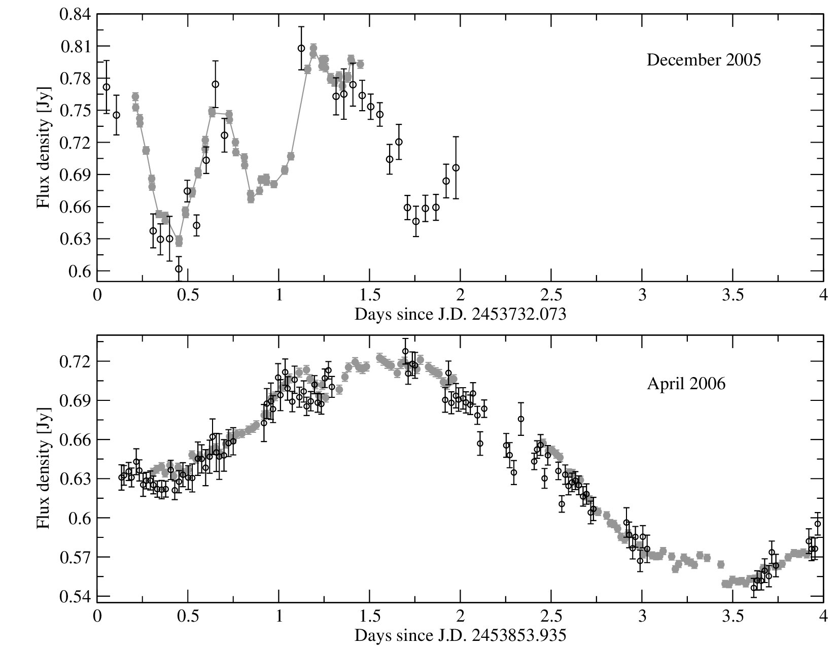 Figure 1
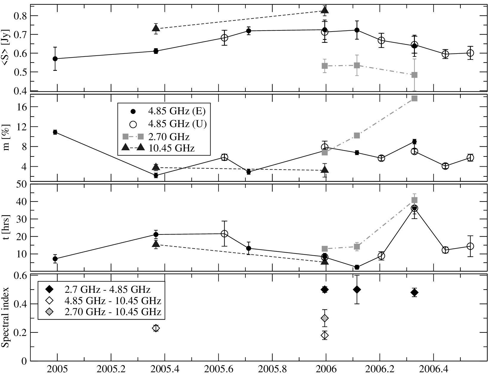 Figure 2
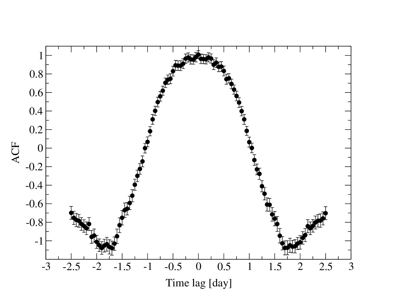 Figure 3
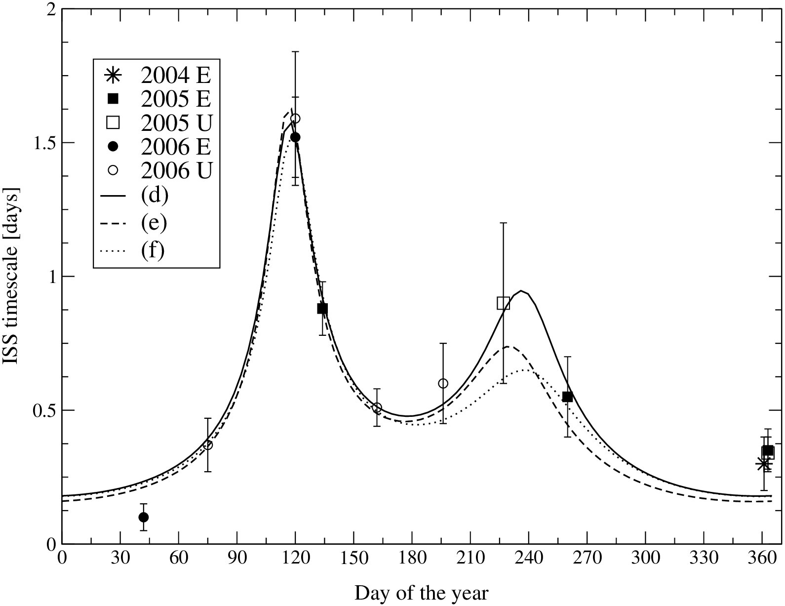 Figure 4
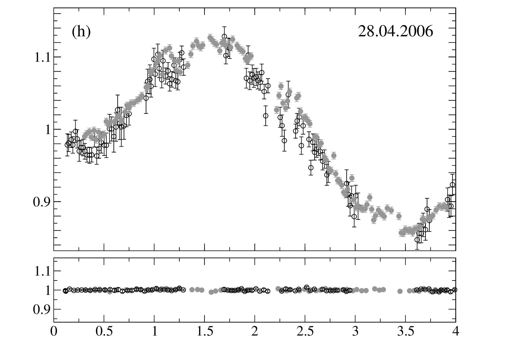 Figure 5
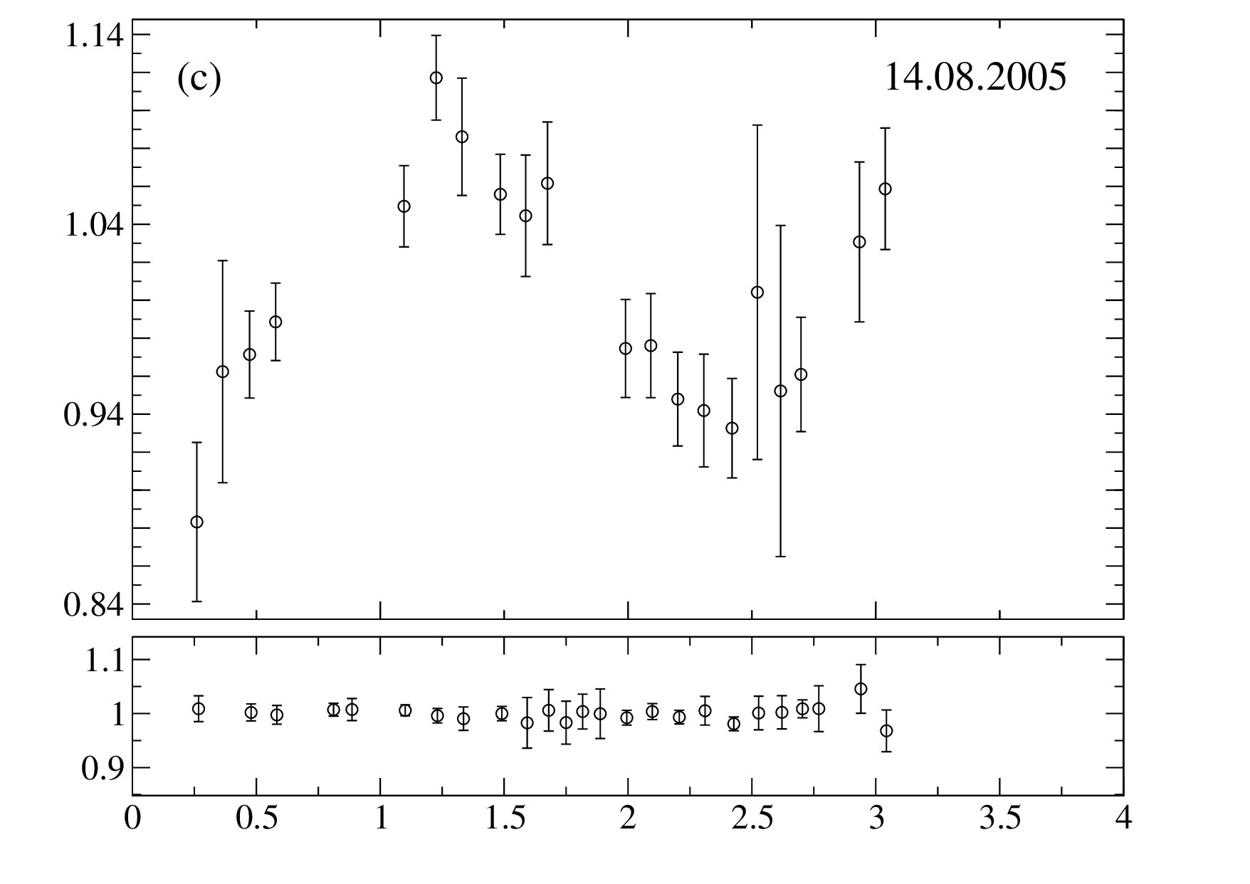 Figure 6
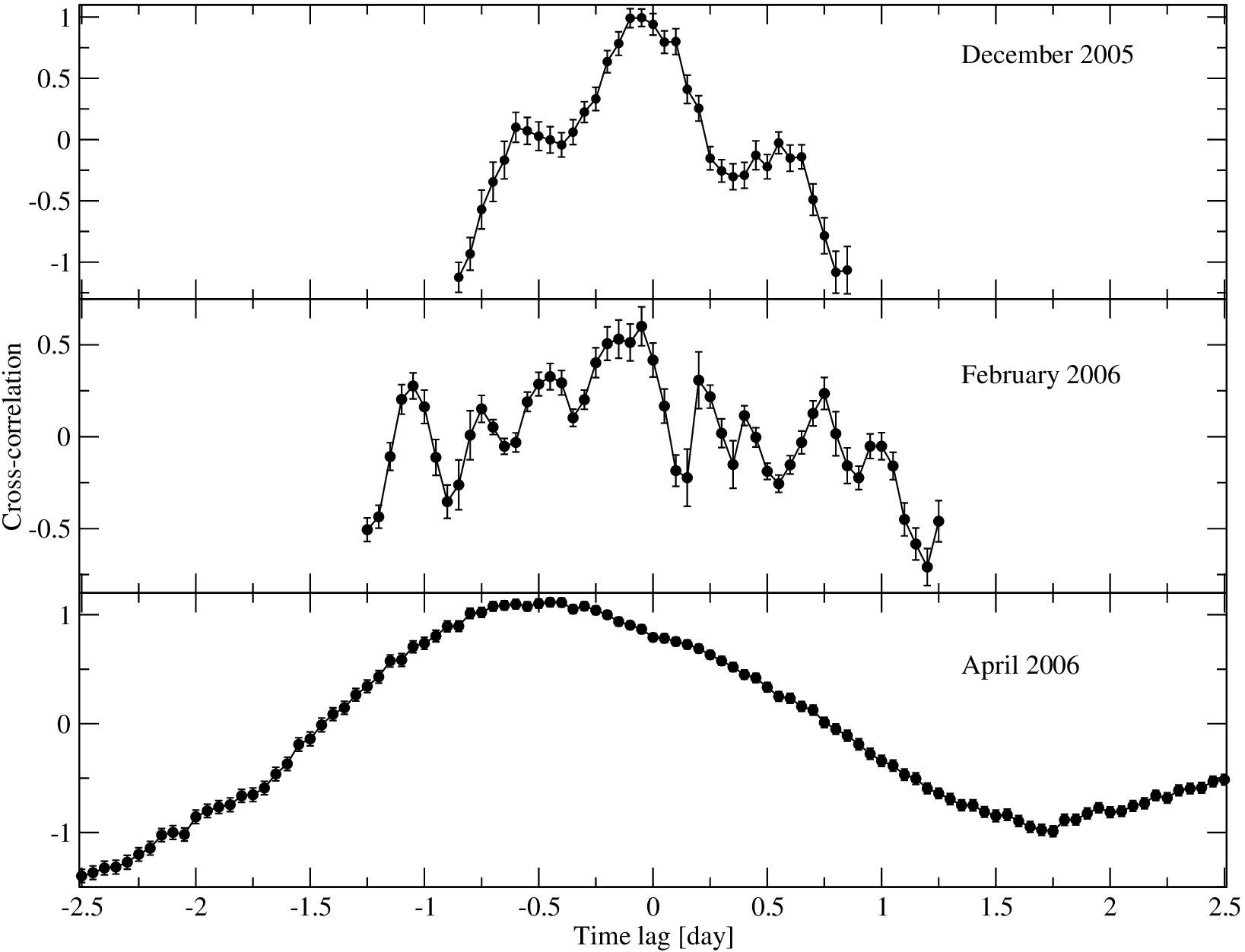 Figure 7
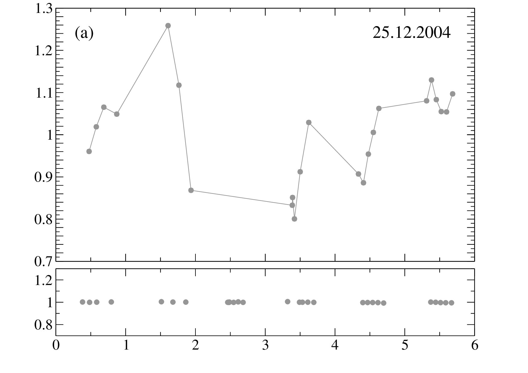 Figure 8
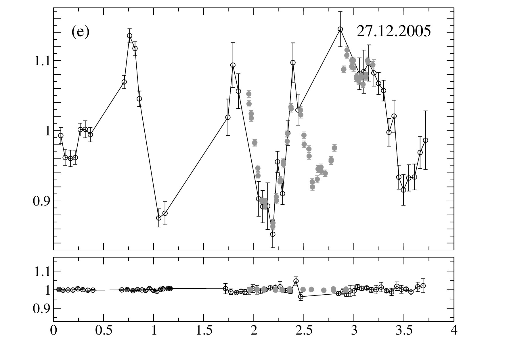 Figure 9
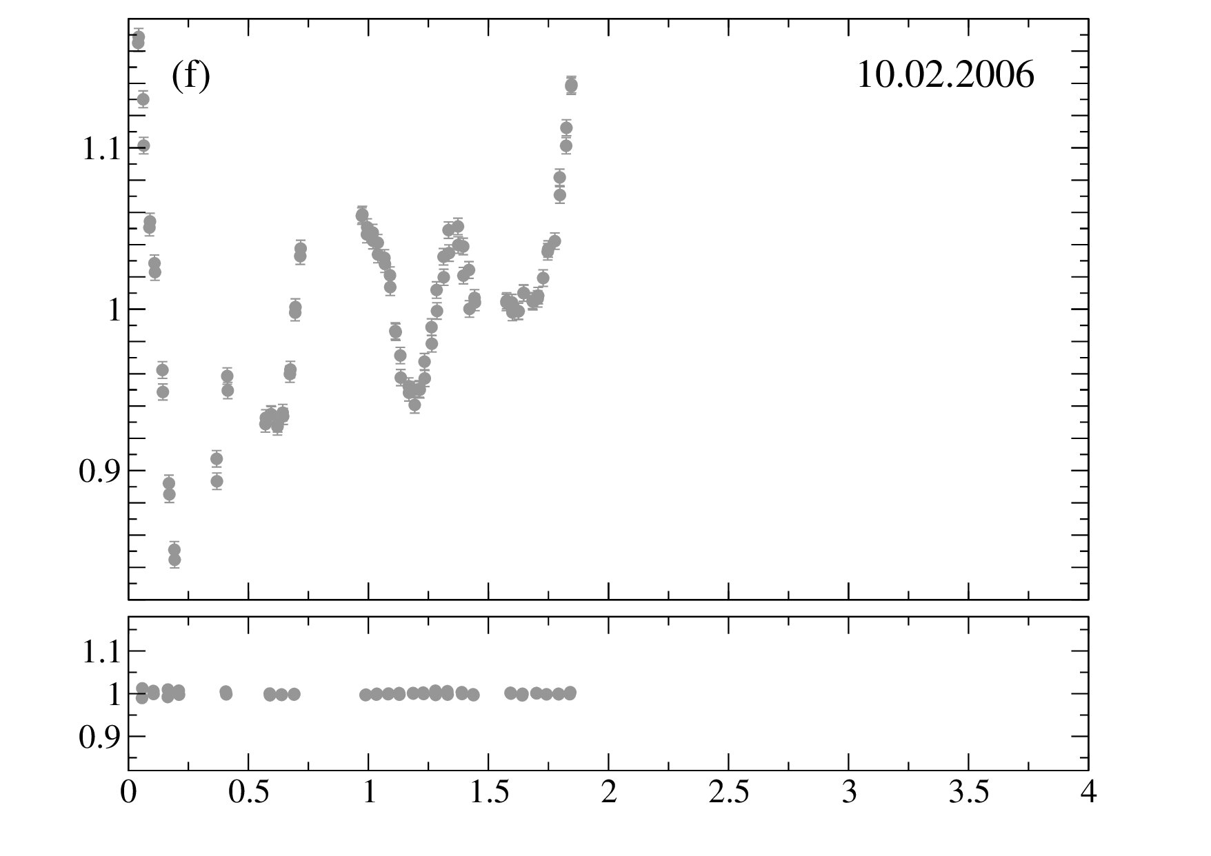 Figure 10
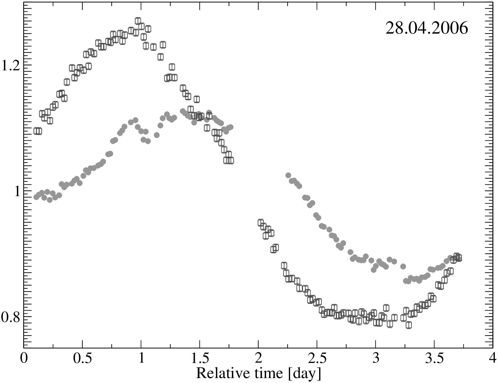 Figure 11
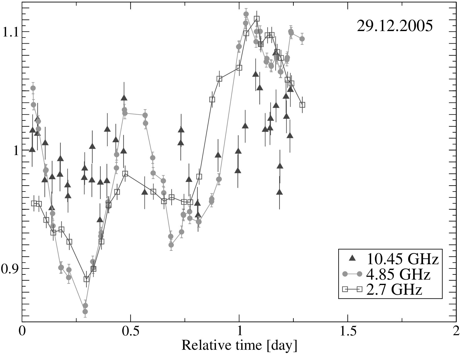 Figure 12
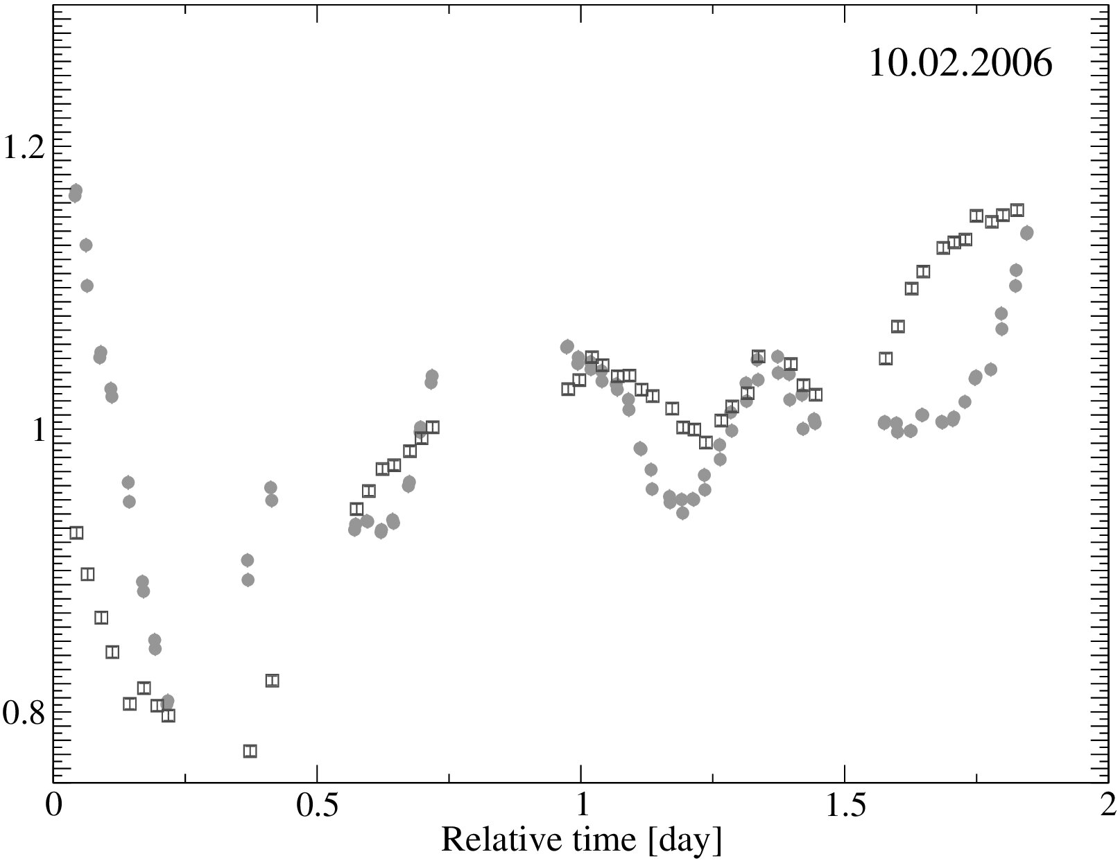 Figure 13
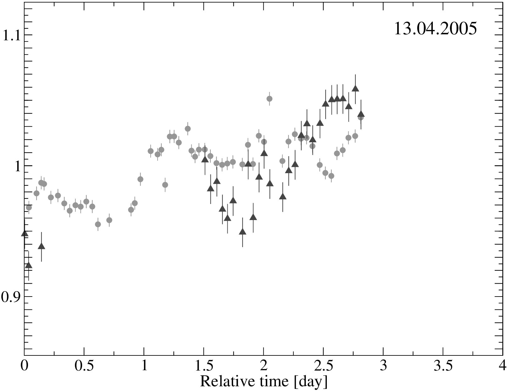 Figure 14
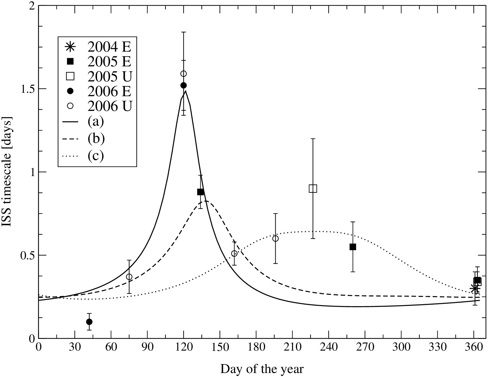 Figure 15
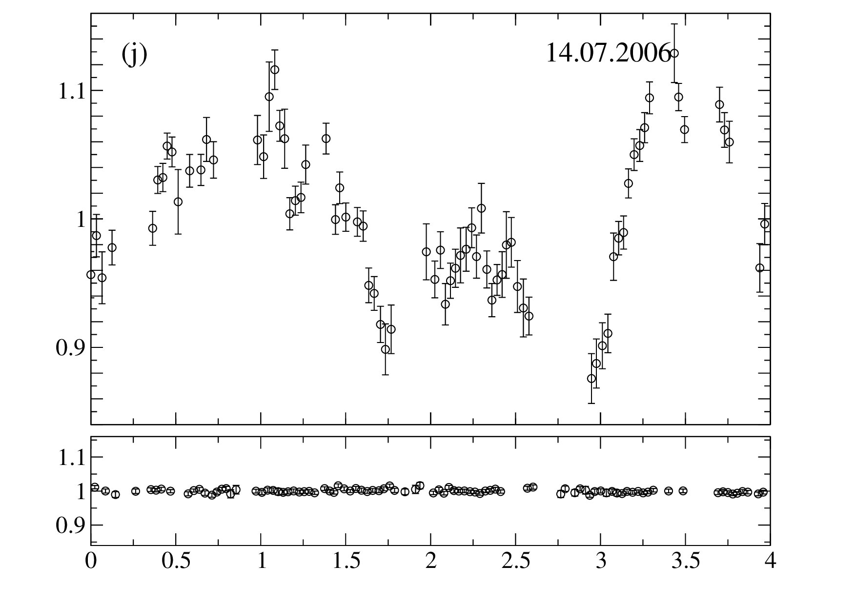 Figure 16
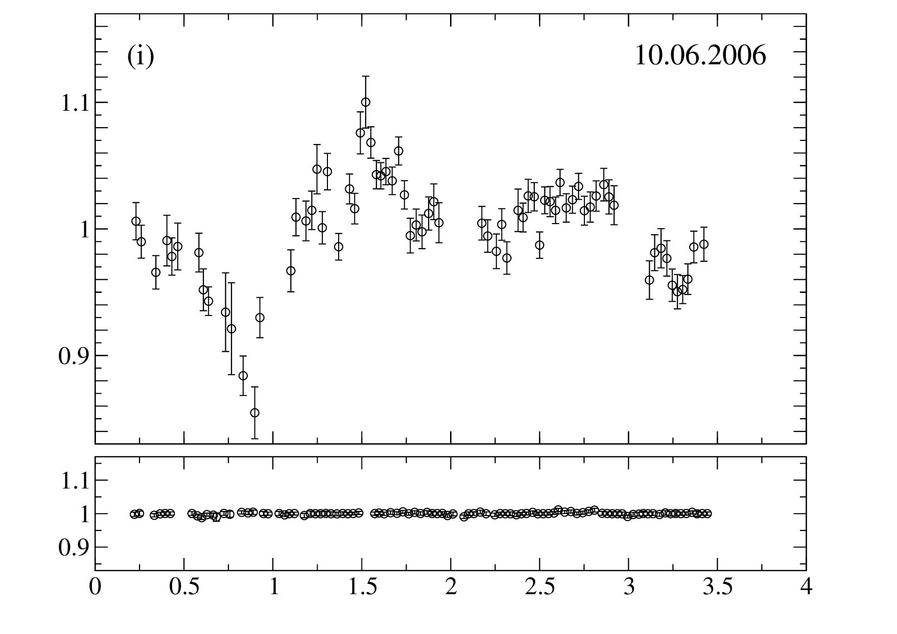 Figure 17
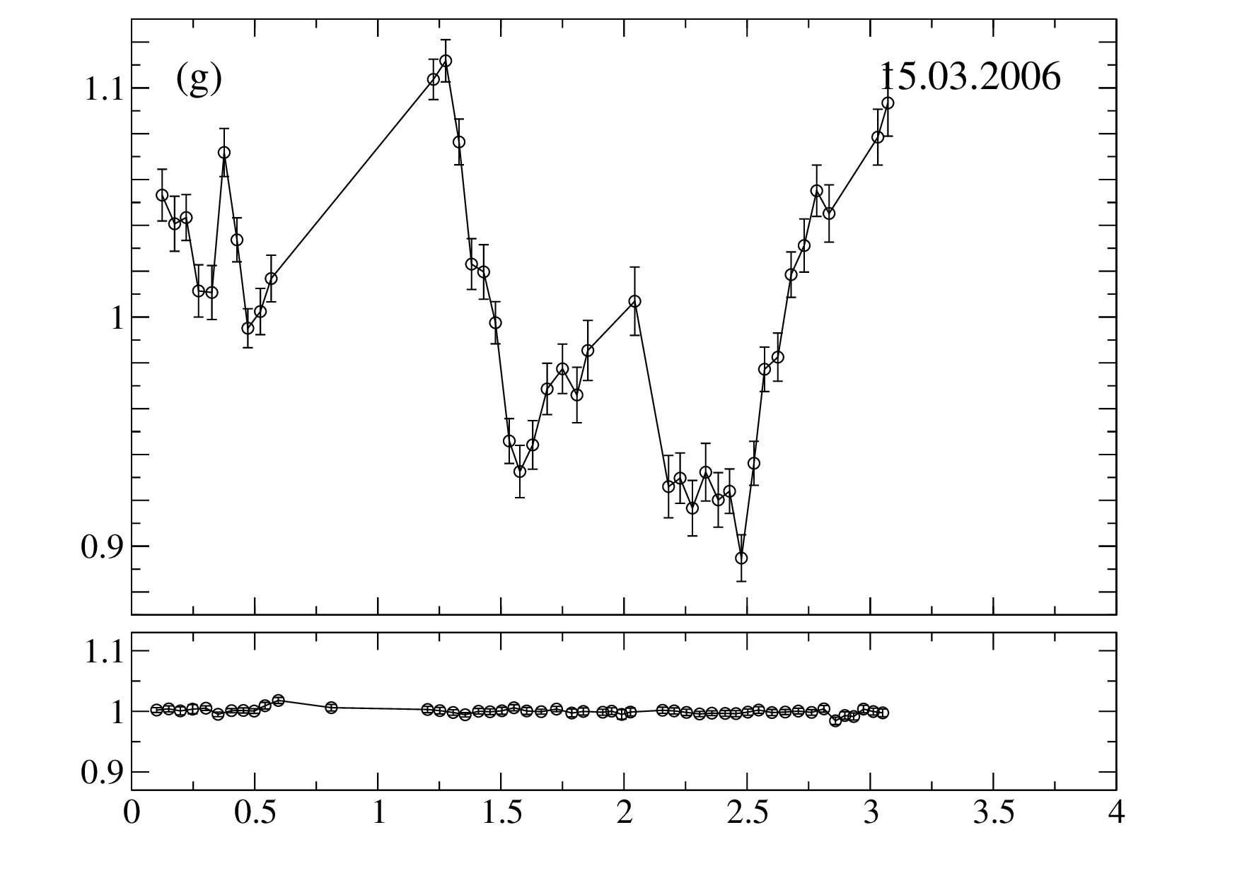 Figure 18
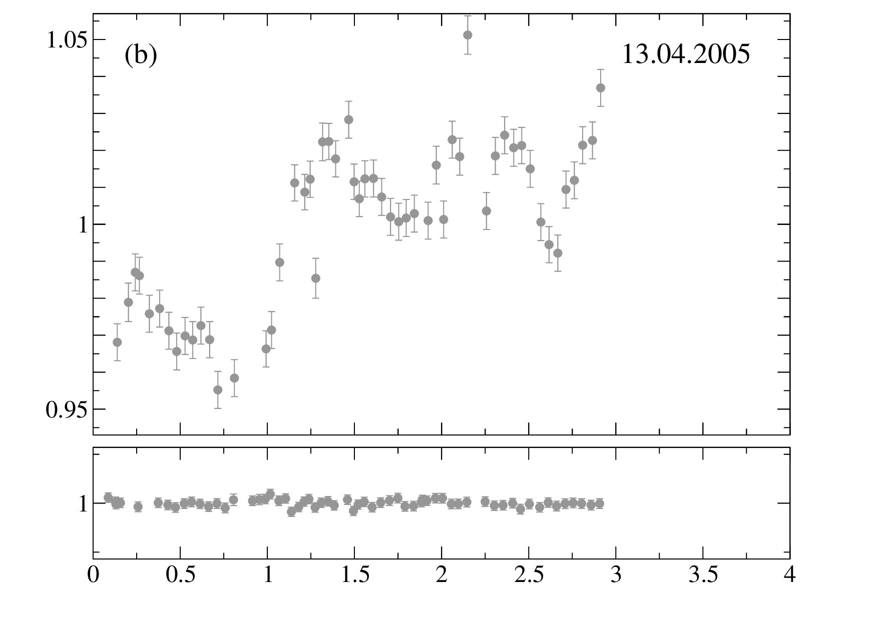 Figure 19
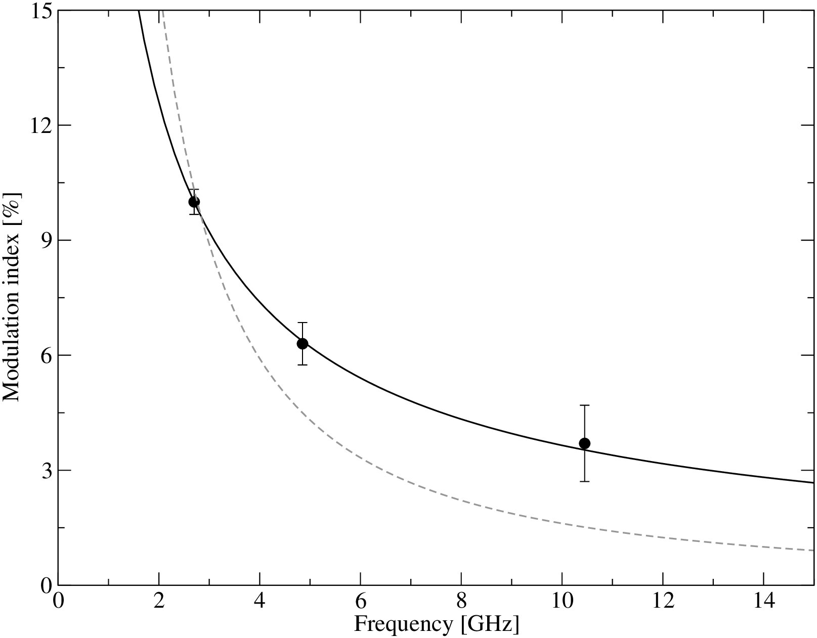 Figure 20
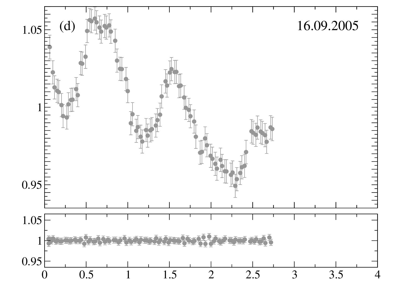 Figure 21
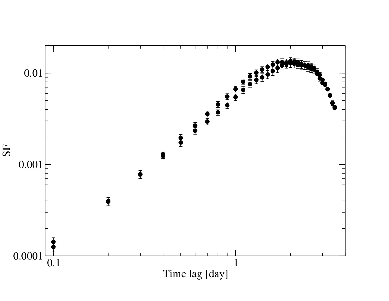 Figure 22
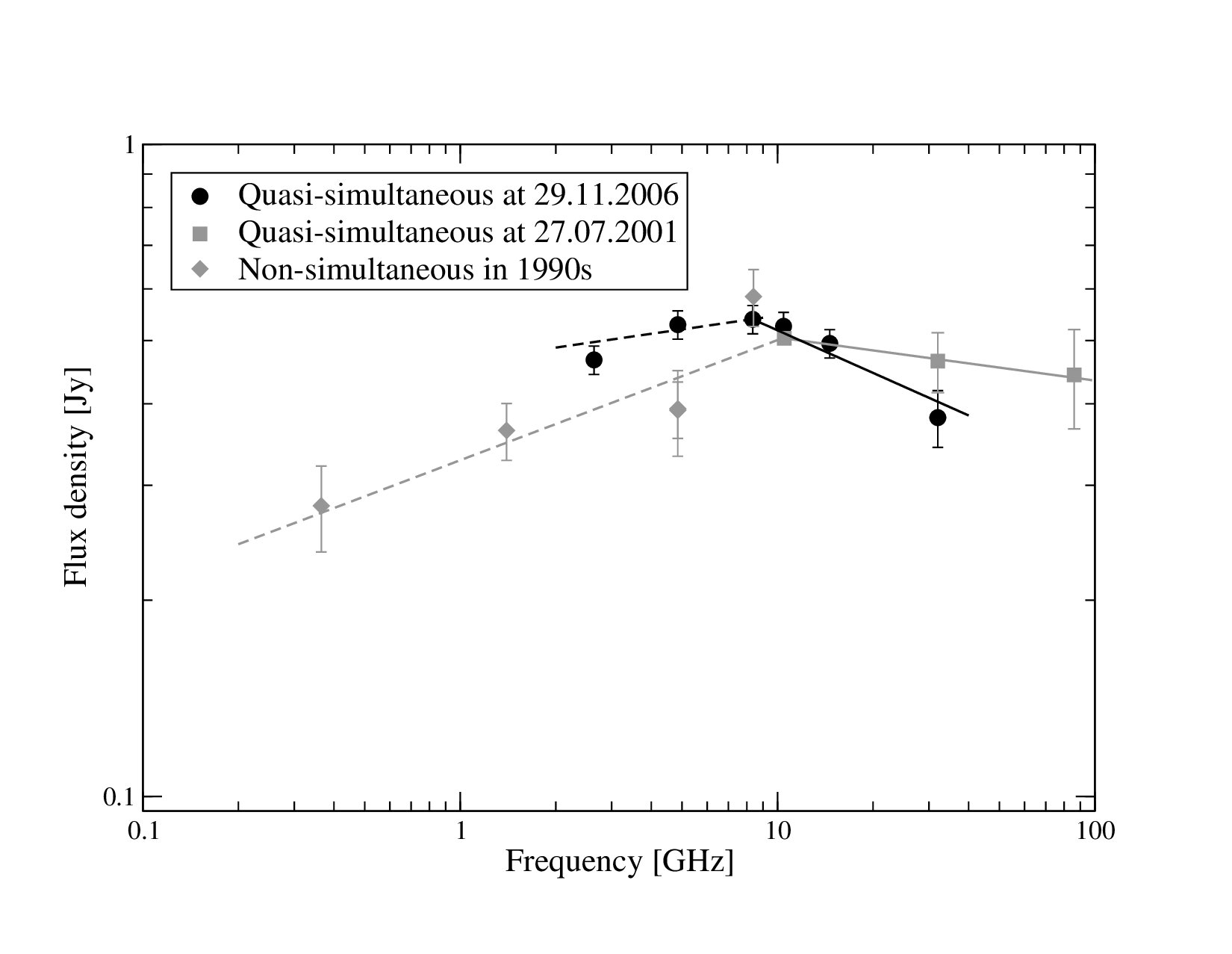 Figure 23
| Epoch | R.T. | Duration | Sampling | ||
|---|---|---|---|---|---|
| [GHz] | [h] | points/hr | |||
| 25-31.12.2004 | E | 4.85 | 125 | 0.2 | (a) |
| 13-16.05.2005 | E | 4.85 | 67 | 0.8 | (b) |
| 13-16.05.2005 | E | 10.45 | 35 | 0.8 | |
| 14-17.08.2005 | U | 4.85 | 67 | 0.4 | (c) |
| 16-19.09.2005 | E | 4.85 | 64 | 1.4 | (d) |
| 27-31.12.2005 | U | 4.85 | 87 | 0.5 | (e) |
| 29-30.12.2005 | E | 2.70 | 29 | 1.0 | |
| 29-30.12.2005 | E | 4.85 | 30 | 2.0 | (e) |
| 29-30.12.2005 | E | 10.45 | 30 | 1.4 | |
| 10-12.02.2006 | E | 2.70 | 43 | 1.1 | |
| 10-12.02.2006 | E | 4.85 | 43 | 2.0 | (f) |
| 15-18.03.2006 | U | 4.85 | 71 | 0.6 | (g) |
| 28.04-02.05.2006 | E | 2.70 | 86 | 1.7 | |
| 28.04-02.05.2006 | E | 4.85 | 86 | 1.4 | (h) |
| 28.04-02.05.2006 | U | 4.85 | 94 | 1.1 | (h) |
| 10-13.06.2006 | U | 4.85 | 77 | 0.9 | (i) |
| 14-18.07.2006 | U | 4.85 | 95 | 0.8 | (j) |
| Name | [Jy] | [Jy] | [Jy] |
|---|---|---|---|
| 3C 48 | 9.32 | 5.48 | 2.60 |
| 3C 286 | 10.56 | 7.48 | 4.45 |
| 3C 295 | 12.19 | 6.56 | 2.62 |
| NGC 7027 | 5.48 |
| Starting date | R.T. | N | m | ||||||||||
|---|---|---|---|---|---|---|---|---|---|---|---|---|---|
| of observation | [GHz] | [%] | [Jy] | [Jy] | [%] | [%] | [day] | [day] | [day] | ||||
| (a) | 25.12.2004 | 4.85 | E | 0.4 | 24 | 0.570 | 0.062 | 10.9 | 32.6 | 000The time-scale obtained from the SF analysis was not consistent with the light-curve. | |||
| (b) | 13.05.2005 | 4.85 | E | 0.5 | 54 | 0.611 | 0.013 | 2.2 | 6.4 | ||||
| 13.05.2005 | 10.45 | E | 0.6 | 29 | 0.730 | 0.028 | 3.8 | 11.2 | |||||
| (c) | 14.08.2005 | 4.85 | U | 0.6 | 20 | 0.682 | 0.040 | 5.9 | 17.5 | ||||
| (d) | 16.09.2005 | 4.85 | E | 0.5 | 91 | 0.719 | 0.021 | 2.9 | 8.6 | ||||
| (e) | 27.12.2005 | 4.85 | U | 1.2 | 40 | 0.713 | 0.056 | 7.9 | 23.4 | ||||
| (e) | 29.12.2005 | 4.85 | E | 0.4 | 64 | 0.725 | 0.052 | 7.2 | 21.5 | ||||
| 29.12.2005 | 2.70 | E | 0.3 | 31 | 0.524 | 0.036 | 6.8 | 20.4 | |||||
| 29.12.2005 | 10.45 | E | 1.4 | 46 | 0.826 | 0.027 | 3.2 | 8.7 | |||||
| (f) | 10.02.2006 | 4.85 | E | 0.4 | 96 | 0.723 | 0.049 | 6.8 | 20.3 | ||||
| 10.02.2006 | 2.70 | E | 0.3 | 47 | 0.526 | 0.054 | 10.2 | 30.6 | 000 are much longer than those derived from the ACF and the light-curve. There is an indication of an additional plateau in the SF at a time lag of day. This agrees well with the other two values of the timescale. | ||||
| (g) | 15.03.2006 | 4.85 | U | 0.5 | 40 | 0.668 | 0.038 | 5.7 | 16.9 | ||||
| (h) | 28.04.2006 | 4.85 | U | 0.5 | 104 | 0.645 | 0.045 | 7.03 | 21.04 | ||||
| (h) | 28.04.2006 | 4.85 | E | 0.5 | 131 | 0.639 | 0.057 | 9.0 | 27.0 | ||||
| 28.04.2006 | 2.70 | E | 0.4 | 137 | 0.484 | 0.085 | 17.7 | 53.0 | |||||
| (i) | 10.06.2006 | 4.85 | U | 0.5 | 72 | 0.595 | 0.024 | 4.1 | 12.2 | 000The time-scales estimations are based upon the variations observed during the first one and half day of the observation. During the last two days the flux-density variations were much more reduced (see Fig. 4 (i) subplot). | |||
| (j) | 14.07.2006 | 4.85 | U | 0.7 | 75 | 0.601 | 0.035 | 5.8 | 17.2 |
| (a) | 1 (fixed) | 0 (fixed) | 4.6 | |||
|---|---|---|---|---|---|---|
| (b) | 1 (fixed) | 0 (fixed) | 4.1 (8.3) | |||
| (c) | 1 (fixed) | 0 (fixed) | 3.0 (13.3) | |||
| (d) | 3.0 | |||||
| (e) | (fixed) | 2.3 | ||||
| (f) | 2.8 |
| SM | ||||
| [pc] | [mas] | [mas] | ||
| (a) | ||||
| (b) | ||||
| (c) | ||||
| (d) | ||||
| (e), (f) |
Peer Reviews
No public reviews on file for this paper yet. If you reviewed it on a platform where reviews are public (OpenReview, ICLR, NeurIPS, ICML), you can paste yours below so the community can read it here.
Videos
No videos yet. Explain this paper in a talk, walkthrough, or lecture? Add one.
11institutetext: Max-Planck-Institut für Radioastronomie (MPIfR), Auf dem Hügel 69, 53121, Bonn, Germany 22institutetext: Hungarian Academy of Sciences (HAS) Research Group for Physical Geodesy and Geodynamics, Budapest, Hungary 33institutetext: Urumqi Observatory,the National Astronomical Observatories, the Chinese Academy of Sciences, Urumqi 830011, PR China 44institutetext: National Astronomical Observatories, Chinese Academy of Sciences, Beijing 100012, PR China
The IDV source J 1128+5925, a new candidate for annual modulation?
K. É. Gabányi 1122
N. Marchili 11
T. P. Krichbaum 11
S. Britzen 11
L. Fuhrmann 11
A. Witzel 11
J. A. Zensus 11
P. Müller 11
X. Liu 33
H. G. Song 33
J. L. Han 44
X. H. Sun 44 [email protected]
(Received / Accepted )
Abstract
*Context. *Short time-scale radio variations of compact extragalactic radio sources, known as IntraDay Variability (IDV), can be explained in at least some sources by a source-extrinsic effect, in which the variations are interpreted as scintillation of radio waves caused by the turbulent interstellar medium of the Milky Way. One of the most convincing observational arguments in favour of propagation-induced variability is the so called “annual modulation” of the characteristic variability time-scale, which is due to the orbital motion of the Earth. So far there are only two sources known, which show such a well-defined seasonal cycle, a few more sources with fewer data can be regarded as possible candidates for this effect. However, source-intrinsic effects, such as structural variations, can also cause the observed changes of the variability time-scale. Data for the new, recently discovered and highly variable IDV source J 1128+5925 are presented.
*Aims. *We study the frequency and time dependence of the IDV in this compact quasar. We measure the characteristic variability time-scale of the IDV throughout the year, and analyze whether the observed changes in the variability time-scale are consistent with annual modulation. Assuming a radio wave propagation effect as origin, we are able to constrain some physical properties (such as distance, scattering-strength and possible anisotropy) of the “plasma” screen, which may cause the scintillation.
*Methods. *We monitored the flux density variability of J 1128+5925 with dense time sampling between 2.7 and 10.45 GHz. We observed with the 100 meter Effelsberg radio telescope of the Max-Planck-Institut für Radioastronomie (MPIfR) at 2.70 GHz, 4.85 GHz, and 10.45 GHz, and with the 25 meter Urumqi radio telescope (China) at 4.85 GHz. From ten observing sessions, each of several days in duration and performed between 2004 – 2006, we determine the variability characteristics and time-scales and investigate these in view of possible scintillation and annual modulation.
*Results. *The observed pronounced changes of the variability time-scale of J 1128+5925 are modelled with an anisotropic annual modulation model. The observed frequency dependence of the variation is in good agreement with the prediction from interstellar scintillation. Adopting a simple model for the annual modulation model and using also the frequency dependence of the IDV, we derive a lower limit to the distance of the scattering screen and an upper limit to the scintillating source size. The latter is found to be consistent with the measured core size from Very Long Baseline Interferometry (VLBI).
Key Words.:
quasars: individual: J 1128+5925 - scattering - radio continuum: galaxies - ISM: structure
††offprints: K. É. Gabányi,
1 Introduction
The so-called IntraDay Variability (IDV) of compact flat-spectrum radio sources (quasars and blazars) was discovered in the mid-eighties by Witzel et al. (1986) and Heeschen et al. (1987). If interpreted as being source intrinsic, the short variability time-scale (of 1–2 days) would imply - through causality and light-travel time arguments - extremely small sizes of the emitting regions (arcsecond-scale), leading to very large apparent brightness temperatures (in the range of K). This is far in excess of the inverse-Compton limit of K (Kellermann & Pauliny-Toth 1969) and would require with the assumption of a spherical geometry excessively large Doppler boosting factors ( ). In somewhat special, non-spherical source geometries (such as cylindrical shock-in-jet models e.g. Qian et al. 1996a, b, 1991; Spada et al. 1999), the requirements for the Doppler factor would be less extreme. Alternatively, coherent processes and collective plasma emission (Benford 1992; Lesch & Pohl 1992), or a short time intrinsic violation of the inverse Compton limit (Slysh 1992) are processes used to explain IDV.
While so far no direct other observational evidence exists for the assumption of such extremely large Doppler factors, the interpretation of IDV via source extrinsic effects appears to be very successful, and in particular explains the very fast (hourly) variations seen in some extremely rapid IDV sources (e.g.: Dennett-Thorpe & de Bruyn 2000). In this source-extrinsic interpretation (e.g.: Rickett 1990), the observed IDV is completely caused by interstellar scintillation (ISS) of radio waves passing through the turbulent plasma of the Milky Way (propagation effect). However, the emission and source structure of compact extragalactic radio sources (quasars, blazars) is known to vary also intrinsically on almost every time scale, from minutes to years. Thus it is very difficult to discriminate between a source intrinsic and a source extrinsic origin of IDV at radio-bands.
One of the most convincing arguments in favour of a source extrinsic explanation of IDV is the so called annual modulation of the variability time-scale. An annual cycle in the observed variability time-scale is caused by the variations of the relative velocity vector between the scattering screen and the velocity of the Earth as the Earth orbits around the Sun (Dennett-Thorpe & de Bruyn 2003). Such seasonal cycles are seen in two IDV sources: J 1819+3845 (Dennett-Thorpe & de Bruyn 2003) and PKS 1257-326 (Bignall et al. 2003). In a few of other IDV sources, such as PKS 1519-273 (Jauncey et al. 2003), B 0917+624 (Rickett et al. 2001; Jauncey & Macquart 2001), PKS 0405-385 (Kedziora-Chudczer 2006) and S5 0954+658 (Fuhrmann et al. in prep., 2007), the observed variability timescales do not show such a clear effect, and a possible seasonal pattern is either not present or is smeared out. For two sources, B 0917+624 (Fuhrmann et al. 2002) and PKS 0405-385, so called episodic IDV (e.g. Kedziora-Chudczer 2006) is observed, where previously observed pronounced IDV, either temporarily disappears (PKS 0405-385), or even ceases (B 0917+624). This makes it difficult to prove beyond doubt the existence of any annual modulation pattern. We note that such episodic IDV can also be due to changes of the source structure (i.e. expansion of previously scintillating structure components) or due to changes in the properties of the scattering plasma.
The other observational argument for an extrinsic explanation of IDV is the “time-delay measurements”, where a time delay is measured between the IDV pattern arrival times at two telescopes. Such time delay of the variability pattern was observed in PKS 0405-385 between the Australia Telescope Compact Array (ATCA) and the Very Long Array (VLA) Jauncey et al. (2001), in J 1819+3845 between the Westerbork Synthesis Radio Telescope (WSRT, Netherlands) and the VLA (Dennett-Thorpe & de Bruyn 2002), and in PKS 1257-326 between the ATCA and the VLA (Bignall et al. 2006). These delay measurements, when combined with the observations of the annual modulation cycle yield constraints to the velocity, geometry and the distance of the plasma causing the scintillation. The time delay measurements are feasible only for rapidly varying IDV sources, where the variability time scale is significantly shorter than the duration of the observing interval. These so called fast scintillators have characteristic variability time-scales of hours or less than an hour. In contrast, the variability time-scales of classical type II IDV sources (Heeschen et al. 1987) are much longer, typically two days, and so time-delay measurements cannot be conducted for these sources.
To establish convincingly an annual modulation pattern, the source has to be observed regularly during the course of the year and for several years. To facilitate the measurement of a characteristic variability time-scale, the duration of an individual IDV session must be long enough, so that several “scintillation” events (“scintles”) can be observed. Within the scheduling constraints of large observatories, the regular observations of fast scintillators, which vary on time-scales of a few hours or less, is easier to perform than for the slower, classical type II IDV sources. For these sources throughout the year regularly performed IDV observations (each lasting at least 3-4 days) cannot be performed with an oversubscribed telescopes, like the MPIfR 100 meter Effelsberg radio telescope. The search for annual modulation in classical type II sources has to invoke other radio telescopes, which can provide more observing time.
In this paper, we present ten epochs of IDV observations for a recently discovered and rapidly variable radio source GB6 J 1128+5925 (henceforth referred to as J 1128+5925): six epochs measured with the MPIfR 100 meter Effelsberg radio telescope at wavelengths 2.8 cm, 6 cm and 11 cm, and six epochs measured with the 25 meter radio telescope in Urumqi (China) at 6 cm wavelength. These observations were aimed to study the IDV characteristics and to measure the IDV time-scale throughout the year.
J 1128+5925 is a radio quasar at a redshift (Sowards-Emmerd et al. 2005), the 2000.0 epoch equatorial coordinates of J 1128+5925 are and (Fey et al. 2004).
The radio spectrum of J 1128+5925 was observed at several dates and is shown in Fig. 1. The spectrum peaks between 8 GHz and 10 GHz. Between 0.365 GHz and 8.4 GHz, a spectral index based on non-simultaneous data from the literature (Patnaik et al. (1992); Gregory & Condon (1991); Becker et al. (1991); White & Becker (1992) and Douglas et al. (1996)) of 111The spectral index is defined as: is measured. Quasi-simultaneous observations performed with the Effelsberg radio telescope and the Plateau de Bure interferometer of the Insititut de Radio Astronomie Millimétrique (IRAM) in 2001 yield a flat high frequency spectrum, with spectral index . Quasi-simultaneous measurements performed in 2006 show some spectral variability when compared to earlier observations, now yielding below the turnover frequency, and above this turnover. The spectral shape and variability is consistent with an inhomogeneous synchrotron self-absorbed compact radio source, which undergoes some long-term variability.
In the following we describe the organization of the paper. In Sect. 2, we summarize the observational details, in Sect. 3 we describe the basic methods used in the variability analysis of the data, in Sect. 4 we present the results and discuss them in the framework of the annual modulation scenario. Sect. 5 contains a summary and conclusion.
The following cosmological parameters were used throughout this paper: .
2 Observations and data reduction
The observations were performed with the MPIfR 100 meter Effelsberg radio telescope at centre frequencies 2.70 GHz (11 cm), 4.85 GHz (6 cm) and 10.45 GHz (2.8 cm), and with the Urumqi radio telescope at 4.85 GHz. The 6 cm receiver, a new backend and a new driving program for the Urumqi telescope was provided by the MPIfR. A detailed technical description of the 6 cm receiver system and the radio telescope are given in e.g. Sun et al. (2007).
J 1128+5925 has been observed at 10 different epochs, which are inhomogenously distributed over a year interval between December 2004 and July 2006. In two epochs (December 2005 and April 2006), the Urumqi and Effelsberg telescopes observed quasi-simultaneously, to allow for checks of the consistency of the flux-density variability seen with the two telescopes. The details of the observations are summarized in Table 1.
At both telescopes, the flux density measurements were performed using the cross-scan technique, in which the telescope was repeatedly moved over the source position in azimuth (Az) and in elevation (El) direction. Four to eight of these slews (sub-scans) in each driving direction formed a scan, which, because of the point-like brightness distribution of the source, is of Gaussian shape. After subtraction of a linear baseline, which removes residual system temperature drifts during a sub-scan, a Gaussian curve was fitted to each of the resulting slices across the source. The peak amplitude of the Gaussian yields a measure of the antenna temperature and of the source strength. The on-source integration time from the 4–8 subscans was found to be adequate to obtain flux-density measurements with a signal-to-noise ratio of SNR at all observing frequencies, which provides sufficient measurement accuracy.
The Effelsberg receivers at 6 cm and 2.8 cm are dual-horn beam-switch systems, which allow to observe simultaneously the source and nearby blank sky (meaning, without the source). The immediate subtraction of the two signals removes the atmospheric fluctuations from the source signal. For a detailed description see e.g. Heeschen et al. (1987) and Kraus et al. (2003).
In contrast to Effelsberg, the 6 cm at Urumqi measured with a single horn only, therefore the fluctuating weather effects could not be subtracted. This reduces the measurement accuracy when the weather is not optimal, and in the presence of rain or rapidly moving clouds led to data, which could not be used for the further data analysis (data removed by manual data editing).
In the next step, the amplitudes of the Gaussian fits to the individual sub-scans were independently averaged in each driving direction (Az, El), and small corrections for the residual telescope pointing errors were applied. In the last step the so corrected amplitudes from both driving directions were averaged together, yielding a single antenna temperature measurement for each source and scan.
The next step of the data reduction is to correct for the systematic elevation dependent gain variations. Elevation dependent effects mainly originate from the gravitational deformation of the dish, which causes variations of the telescope gain with changing elevation. A polynomial correction was determined using the combined gain-elevation curves obtained from the non-variable calibrator sources.
After this, the time-dependent gain variations must be corrected. These time-dependent effects are mainly caused by the changing weather conditions during the observations, by long-term gain fluctuations of the receivers and from thermal gradients in the telescope. These effects can be corrected using a gain-time transfer function derived from measurements of several secondary calibrator sources (e.g. B 0836+710 and B 0951+699), which are observed with the same duty cycle as the target sources. Since these sources do not vary on short (IDV) timescales, their measured amplitude variations can be used to determine the time dependent gain variation of the whole system (telescope + receiver + atmosphere) with high ( 0.8 %) accuracy. The observation of more than one of these secondary calibrators ensures the correctness of the assumption of non-variability of each secondary calibrator.
In the last step, the measured flux densities were then tied to the absolute flux-density scale, which was determined from repeated observations of the primary calibrators e.g. 3C 48, 3C 286, 3C 295 and NGC 7027 and using the flux-density scale of Baars et al. (1977) and Ott et al. (1994). In Table 2 we summarize the used flux densities for each primary calibrator.
The residual scatter in the measured flux densities of primary and secondary calibrator provides a very good and also conservative estimate of the overall calibration accuracy. We note that this is mainly limited by the systematic time variations of the overall system response, and not by the individual flux measurement, which is of high SNR. These time dependent gain variations are monitored through the observed variations of the primary and secondary calibrator fluxe densities. After correction of all afore-mentioned gain effects, the residual variability of the calibrators yields a very reliable estimate of the measurement accuracy, and furthermore does not depend on a-priori assumptions on receiver stability and telescope gain. We quantify the overall measurement accuracy using the variability index of the secondary calibrators, where is the weighted average ratio of the standard deviations to the mean flux density for all calibrators. Thus, the uncertainty of an individual flux density measurement is be given by . The values for for each experiment are given in Col. 5 of Table 3. Typically, one obtains for Effelsberg % at 2.70 GHz, % at 4.85 GHz, and % at 10.45 GHz, mainly reflecting the fact that the atmosphere limits the measurement accuracy towards higher observing frequencies.
At Urumqi one obtains at 4.85 GHz typically %. A somewhat larger value of % is observed in December 2005, which is due to bad weather conditions (rain and snow).
2.1 Comparing the Effelsberg and the Urumqi data
The direct comparison of the variability curves obtained with the 100 m Effelsberg and 25 m Urumqi telescope in two quasi-simultaneous observing sessions (Dec. 2005, April 2006, see Fig. 2, and Tab. 3), shows a very good agreement of the variability curves measured at both telescopes and demonstrates that the 25 m Urumqi telescope is well suited for IDV studies. The small differences seen in the rms-scatter of both data trains are likely to result from some fundamental differences between the two observatories:
- •
The 100 m Effelsberg dish uses the homology principle, the 25 m Urumqi telescope does not. Consequently, the gravitational deformation as a function of elevation is different for both dishes, resulting in a lower aperture efficiency and steeper gain-elevation curves of the Urumqi telescope.
- •
While for the 100 m Effelsberg telescope, the focus position is automatically adjusted at each elevation and also allows manual displacement and refocusing at any time (day, night), the focus in the Urumqi telescope is at a fixed position, not allowing for additional focus corrections. This leads to stronger variations of the overall time dependent gain.
- •
At 4.85 GHz, Effelsberg uses a dual-horn beam-switch receiver, while at Urumqi a single horn total power receiver is used. The Urumqi data are therefore more affected by the weather than the Effelsberg data. At Urumqi, this results in a less stable signal, which is probably the main reason for the larger scatter seen in these data.
For the 6 cm observations performed at Urumqi, we used the following secondary calibrators, each of which with a flux density comparable to that of our program sources: B 0836+710 ( Jy), B 0951+699 ( Jy), B 1203+645 ( Jy), B 1128+455 ( Jy), B 1311+678 ( Jy). We find it remarkable that despite a 16 times smaller collecting area of the Urumqi telescope, the achieved measurement accuracy ( % at Urumqi, % at Effelsberg, see Tab. 3) is only times worse than at Effelsberg. This demonstrates that the IDV measurements performed with Urumqi are not limited by the size of the dish and the signal-to-noise ratio, but by the larger fractional errors which are most likely the result of the afore-mentioned three effects.
3 Data analysis
For the variability analysis, we follow earlier work and use a parameterization already introduced by Heeschen et al. (1987) and described in detail in e.g. Quirrenbach et al. (2000).
To decide whether a source can be regarded as variable, we performed a test, which tests the hypothesis whether the light curve can be modeled by a constant function. Sources for which the probability of this hypothesis is less than 0.1% are considered to be variable.
The amount of variability in a light-curve is described by the modulation index and the variability amplitude. The modulation index is defined by , where is the time average of the measured flux density, and is the standard deviation of the mean flux density. (The mean modulation index of the calibrators, describes the overall calibration accuracy, see Sect. 2).
In estimating the errors of the modulation index of the variable source, the statistical effects of a stochastic process have to be taken into account (Cimó 2003). The errors originate from the limited observing time and from the time sampling. If the observing time is much shorter than the characteristic variability time-scale (no clear maximum followed by a minimum can be observed in the light-curve), the variability index is not well defined. The contribution to the statistical error, originating from the length of the observing interval, is proportional to , where is the characteristic variability time-scale and is the total observing time (B. Rickett, priv. comm.). In addition, variability may also exist at times below the mean sampling interval of the measurements. Under-sampled variability also leads to an underestimate of the variability index . Assuming that significant variations may exist between three data-points, the error is given as: , where is the mean sampling interval (Cimó 2003). Both of these effects were taken into account for the calculation of the uncertainty of the modulation index , which was found to range between % and % of the given value of .
Following Heeschen et al. (1987) we define a -variablity amplitude through the noise-bias corrected -value of the modulation index . We define the variability amplitude of a given source with variability index as , where is the mean modulation index of all secondary calibrators, which describes the statistical measurement accuracy during the observation. is set to zero for non-variable sources ().
3.1 Determination of the characteristic variability time-scales
There are many different definitions for the characteristic variability time-scale of IDV used in the literature. E.g. Simonetti et al. (1985) use the structure function of the observed time series to define a characteristic variability time-scale. Rickett et al. (1995) and Rickett et al. (2002) define the variability time-scale by the half-width at half maximum of the autocorrelation function. Macquart & Jauncey (2002) use the half-width at of the maximum of the autocorrelation function (this definition of the so called decorrelation time-scale is adopted from pulsar scintillation studies, see e.g. Cordes 1986). Since IDV light-curves appear often quasi-periodic, resembling some sort of sine-wave pattern, the variability time-scales can also be estimated from the mean peak-to-peak (Kedziora-Chudczer et al. 1997) or peak-to-trough time (Jauncey & Macquart 2001).
To obtain reliable estimates of the variability time-scales present in our data, we derived the time-scales using 3 different methods:
- •
We calculated from the light-curves the average peak-to-trough time (, Col. 12 in Table 3). The errors are calculated from the internal scatter of the different peak-to-trough times found in one data train. In some light curves, the peaks and troughs were not well-defined. In these cases we do not give an error estimate, the time-scales are given in parenthesis in the table.
- •
We calculated the structure function (SF) for each time series and derived the “saturation” time-scale from it. (, Col. 13 in Table 3). The SF is defined as , where is the flux density time-series, is the time-lag and denote time averaging. Above the noise level, the SF rises monotonically and is described by a power law. At large time-lags, the SF reaches its maximum at a “saturation” level, which is proportional to . The intersection of the power-law fit with this “saturation” level defines the characteristic variability time-scale (Beckert et al. 2002). The measurement error for this time-scale is derived from the formal errors of the power law fit and the fit of the “saturation” level (Fuhrmann 2004; Fuhrmann et al. 2007, in prep.).
- •
We also calculated the autocorrelation function (ACF) of the time series, using the method of Edelson & Krolik (1988). The ACF is related to the SF via: . Thus, the time-lag derived from the point where the SF reaches its maximum corresponds to the time-lag at the first minimum of the ACF. The derived time-scales () are given in Col. 14 of Table 3. The error of are determined from the scatter in the positions of the first minimum of the ACF, when calculated with different bin sizes.
Examples of structure functions (SF) and autocorrelation functions (ACF) obtained for J 1128+5925 are displayed in Fig. 3. The functions were derived from the light curve observed at 4.85 GHz with the Effelsberg radio telescope in 28 April 2006. The corresponding light-curve is shown in Fig. 4 in subplot (h).
4 Results
In Figure 4 we show the radio variability curves of J 1128+5925 obtained at 4.85 GHz during December 2004 and July 2006. For each observing date the normalized flux density of J 1128+5925 (top panel) and of a secondary calibrator (B 0836+710, panel below) is plotted versus time (in days). In the plots, the amplitude scale for J 1128+5925 and for the secondary calibrators are similar, visualizing the prominence of the variability seen in J 1128+5925. Here, the peak-to-trough amplitude is found to reach %. The light-curves often appear quasi-periodic (e.g. in 2005 September subplot (d), 2005 April subplot (h)) and show some complexity, indicative of the presence of more than one variability time-scale. The variability characteristics, time-scales and strength of the variability change significantly from epoch to epoch, and sometimes even within a day interval. For example in June 2006 (subplot (i)), where a pronounced trough and peak is followed by a much shallower variations during the last days of the observations.
In Table 3, we summarize the results of the observations of J 1128+5925. We list the variablity parameters for all observing sessions: Column 1 gives a label, which refers to the variability curve shown in Figure 4, col. 2 summarizes the observing date (first day, dd/mm/yyyy), col. 3 the observing frequency, col. 4, the observatory, col. 5 the mean modulation index of the secondary calibrators, column 6 the number of data points obtained for J 1128+5925, col. 7 the mean (time averaged) flux density of J 1128+5925 in this session, col. 8 the standard deviation for the mean flux density, col. 9 the modulation index, col. 10 the variability amplitude, and col. 11 the reduced . For the degrees of freedom considered here, a 99.9 % probability for variability is given, when the reduced exceeds . With in the range of to , the variability of J 1128+5925 is highly significant at all observing dates and frequencies. We note that at 10.45 GHz the variations are somewhat lower. A detailed description and discussion of the frequency dependence of variability is given in Sect. 4.3.
In columns 12, 13, and 14 of Table 3, we summarize the three different estimates of the variability time-scale. The calculation of the variability time-scale is described in detail in Sect. 3.1.
The typical variability time-scales range between days. For each observing epoch and data set, the three different methods reveal similar results and show the internal consistency of the measured variability time-scales.
Adopting a source-intrinsic interpretations for the variability, we can apply the light travel-time argument and derive - via the source size - an apparent brightness temperature. Following Marscher et al. (1979), the angular size (in mas) is obtained from: . Here, is the variability time-scale (in days), is the source redshift, the luminosity distance (in Gpc) and the Doppler factor. This size now can be used to calculate a brightness temperature which, in the case of a Gaussian brightness distribution, is given by: K (e.g. Kovalev et al. 2006). Here is the flux density in Jy, the observing frequency in GHz and the source size in mas.
Even if one uses the longest measured variability time-scale (of 1.7 days as measured in April 2006 at 4.85 GHz), one obtains a brightness temperatures far in excess of the inverse-Compton limit of K. The fastest observed variations (seen in December 2005 and February 2006) imply K. Independent of the use of the inverse Compton brightness temperature limit ( K, Kellermann & Pauliny-Toth 1969) or the equipartition brightness temperature limit ( K, Scott & Readhead 1977; Readhead 1994), this leads to Doppler-boosting factors of a couple of hundreds to thousand, which are necessary to bring the observed brightness temperatures back to these limits.
4.1 Time dependence of the variability
In J 1128+5925, the variability amplitudes and time-scales vary at each observing frequency significantly between the different epochs (see Fig. 4 and Table 3).
The length and sampling of the observations may influence the measurements of these parameters. However, only in some cases are the observed differences due to sampling effects. This is illustrated in the variability curves of December 2005, which despite a different time sampling and and by a factor of two different duration of the observation at Effelsberg and Urumqi still leads to very comparable variability indices, amplitudes and time-scales.
To search for a possible correlation of the IDV with long-term variations of the total flux density, we plot in Fig. 5 the mean flux density, the modulation index, the variability time-scale and the spectral index versus observing epoch. Measurements at different frequencies performed by different telescopes are shown with different symbols.
The variations of the modulation index and of the variability time-scale do not show a correlation with the total flux density. The mean flux densities at 4.85 GHz showed an increase by % until February 2006, over a yr time-scale. This increase is also seen at 10.45 GHz. After this, the 4.85 GHz flux density decreased almost to its original value by July 2006. Unfortunately, we were unable to find additional total flux density monitoring data for J 1128+5925 in the literature, which would allow to us to check if and how the flux density varies on longer time-scales. Clearly, a future flux density monitoring would be helpful.
The spectral index was calculated for those 4 epochs for which we had quasi-simultaneous multi-frequency measurements. We obtained a spectral indices between 4.85 GHz and 10.45 GHz in May 2005 and in December 2005, and between 2.70 GHz and 4.85 GHz in February 2006 and April 2006. We also determined the spectral index using all three frequencies in December 2005. Within the limited amount of multi-frequency data, we do not see pronounced temporal variations in any of these spectral indices. The observations, however, indicate some change of the spectral slope at 4.85 GHz from steep to flat. The data are also consistent with a spectral turnover between 8 GHz and 10 GHz, which is already seen in Fig. 1.
4.2 Annual modulation model
The variability time-scales seen in J 1128+5925 are significantly different at different epochs (Fig. 4 and Table 3). At 4.85 GHz, the changes in the characteristic variability time-scale do not correlate with other parameters of the variability (see Fig. 5). However, it is striking that in two observations separated by one year (December 2004 and 2005) a very similar variability time-scale of days is seen. The robustness of this short variability timescale is independently confirmed by two telescopes (Effelsberg and Urumqi, December 2005).
In Fig. 6, we plot the variability time-scale versus day of the year. Different symbols represent different years of observations: stars for 2004, squares for 2005, circles for 2006. From Fig. 6, the slowest variations occurs around day 120 (end of April to early May, day). Although the number of data points is sparse, the figure shows another “slow-down” of the variability time-scale around day 230 (August, September). In the following, we try to explain this behaviour by two scenarios within the framework of the annual modulation model.
A seasonal cycle of the characteristic variability time-scale can be explained in a model of interstellar scintillation (ISS), where the scattering material is regarded to be located in a thin plasma screen at some distance from the Earth. The orbital motion of the Earth around the Sun leads to annual velocity changes, resulting from the vector addition between the observer’s velocity vector and the velocity vector of the screen. Thus annual modulation is a pure geometrical effect. A low relative velocity between screen and observer results in a prolongation of the observed variability time-scale. Half a year later the two velocity vectors are oriented oppositely. This then leads to a large velocity difference and correspondingly to fast variability (e.g. Bondi et al. 1994; Rickett et al. 2001; Dennett-Thorpe & de Bruyn 2003).
In such a model the free parameters are the components of the velocity vector of the screen in the plane perpendicular to the line of sight, and the scattering length scale (). The scintillation time-scale as a function of the day of the year () then is given as: , where is the relative velocity between the observer and the screen.
In the left panel of Fig. 6 the three different lines represent annual modulation models calculated from three different sets of input parameters. The first curve, (a), is the best fit to the whole dataset and yields a . In an attempt to fit the second “slow-down” of the variability time-scale around day 230, we first excluded the data points at day 120. This gave the slowest variability time-scale and thus determines the height of the first peak. Thus, we obtained curve (b). The of this fit was , however including all the data points yielded . To be able to fit the “slow-down” at day 230 one has to exclude also the measurement at day 134. This is illustrated by curve (c) The of this reduced dataset was , however using all the data points yielded a . To summarize, the first “slow-down” at day 120 is not due to one exceptionally long variability time-scale, but is constrained by two measurements, one obtained in May 2005 and the other in April 2006.
The parameters of the different curves are given in Table 4. In Col. 1, the letters refer to the corresponding curve displayed in Fig. 6. In Col. 2 and 3, the components of the screen velocity are displayed in Right Ascension () and in Declination (). In Col. 4, the scintillation length scale is given. Fig. 6 shows that this annual modulation model can explain only one slow-down of the variability time-scale in one year, but not two.
The previous model assumed an isotropic scintillation pattern. However, in a more general scenario, scintillation patterns could also be anisotropic. This is modelled by introducing some ellipticity. Including the anisotropy of the scintillation pattern introduces two more model parameters: the angular ratio of the anisotropy () and its position angle (). The scintillation time-scale now also depends on the direction of the relative velocity vector (between the Earth and the screen) and how it “cuts” through the elliptical scintillation pattern. Following Bignall et al. (2006), the scintillation time-scale is given as the function of day of the year () by the following expression:
[TABLE]
where is the scintillation length scale. is the relative velocity between the scintillation screen and the observer. As the Earth orbits around the Sun varies annually. denotes the absolute value of . is the unit vector, defining the orientation of the elliptical scintillation pattern, where the angle is measured from East through North. The major and minor axis scale lengths of the scintillation pattern are defined through , and , respectively. We note that in this paper the definition of the time-scale differs from that used by Bignall et al. (2006). This leads to a factor of difference between the scintillation length scale derived here and by Bignall et al. (2006).
In the right panel of Fig. 6 the fits for the anisotropic annual models are displayed. The parameters of the three model curves are summarized in Table 4.
The simple isotropical scintillation model can not explain both, the “slow-down” of the scintillation time-scale at around day 120, and the increase of the variability time-scales measured after day 230. The anisotropic scattering model of Bignall et al. (2006), however, does reproduce both features quite well. Owing to its broader shape and lower modulation, this second “slow-down” around day 230 is not as well determined as the peak around day 120, therefore are the corresponding parameters and are not so well constrained.
In the case of a point source (i.e. a source smaller than the Fresnel angle) the scattering length scale is determined by the Fresnel angle and the distance to the scattering screen. The Fresnel angle is given as , where is the distance to the scattering screen and is the observing frequency. Extragalactic radio sources usually cannot be regarded as point-like in this context, since . Therefore, the scattering length scale is mainly determined by the source size and not by the Fresnel angle (e.g. Goodman 1997; Walker 1998). Therefore, the distance to the screen can be derived from the scintillation length scale with the assumption of an angular source size.
For this, we use the VLBI data obtained for J 1128+5925 through images and Gaussian modelfits. The source was observed with VLBI at 5 GHz in the Caltech-Jodrell Bank Flat-Spectrum Survey (CJF survey, Taylor et al. 1996; Ma et al. 1998, and S. Britzen in prep., 2007). J 1128+5925 is a very compact radio source, with a possible jet-like feature oriented towards the south-west at a position angle of . From circular Gaussian modelfits an upper limit to the VLBI core size of 0.53 mas (in 1992.731) and 0.13 mas (in 1994.702) (S. Britzen, priv. commm.) is obtained.
An independent size estimate is obtained from the turn-over frequency of the radio spectrum of J 1128+5925 (see Fig. 1). Assuming that the observed spectral turn-over is due to synchrotron self-absorption and further assuming energy equipartition between particles and magnetic field, allows to calculate the so called equipartition source size (e.g. Scott & Readhead 1977). Adopting 8.35 GHz as the turnover frequency and using the flux-density measured at this frequency ( Jy), one obtains the equipartition source size via: mas, where is the luminosity distance, the redshift of the source and the Doppler factor. From the CJF survey (Britzen et al. 2007, and in prep.) the Doppler factor is estimated to be . With this one obtains an equipartition size of mas at 8.35 GHz. We now may assume that the source size is inversely proportional to the observing frequency (for discussion see, Sect. 4.3). This leads to an extrapolated source size of mas at 4.85 GHz.
From the definition of the scintillation length scale , and using the above derived upper limit for , we obtain a lower limit to the screen distance. Taking the source size derived from the spectrum of J 1128+5925 ( mas), the calculated lower limits on the screen distance range between pc and pc. Using the source size derived from the modelfits of the CJF survey data ( mas) the lower limits on the screen distances range between pc and pc. At these distances the Fresnel angular scales at 4.85 GHz indeed range between as and as. This confirms our initial assumption of the Fresnel scale being smaller then the source size. Therefore the source cannot be regarded to be point-like.
If we assumed that the source size is smaller than or equal to the Fresnel scale, than the scintillation length-scale is determined by the distance to the scattering screen and the Fresnel angular size. However, in that case the assumed source sizes would be extremely small (as) compared to usual extragalactic source sizes. Assuming a circularly symmetric source with FWHM corresponding to these Fresnel angle values implies a lower limit on the brightness temperature of the order of K.
The modelfits of the CJF survey VLBI data revealed in two epochs (1994.702 and in 1996.646) a secondary (jet?) component at a position angle and relative to the core. These position angles agree remarkably well with the position angle of the anisotropy derived from the anisotropic annual modulation model (). It is therefore possible that the annual modulation and the by the model predicted amplitude and seasonal times of the two major maxima in Figure 6 are related to the VLBI structure and its orientation. At the moment it is unclear, if the agreement between both angles is a chance coincidence. Moreover the VLBI observations of the source were performed ten years before our IDV observations and it is unclear if the jet orientation is persistent over such a long time. To confirm whether the orientation of the source elongation remained constant over time, and whether it is related to the anisotropy seen in the annual modulation pattern, requires further VLBI observations.
A seasonal cycles seen in the variability time-scales of some other IDV sources (such as J 1819+3845 (Dennett-Thorpe & de Bruyn 2003), PKS 1257-326 (Bignall et al. 2003), 1519-273 (Jauncey et al. 2003), B 0917+624 (Rickett et al. 2001; Jauncey & Macquart 2001) and S4 0954+658 (L. Fuhrmann priv. com.)) are similarly explained in the framework of the annual modulation theory. Assuming anisotropy in the scintillation pattern, Dennett-Thorpe & de Bruyn (2003) and Bignall et al. (2006) successfully modeled the annual variations in the characteristic variability time-scales in the extremely fast IDV sources, J 1819+3845 and in PKS 1257-326. The derived screen distances in these sources were less than pc, comparable to the lower limits to the screen distance derived here.
4.3 Frequency dependence of the variability
J 1128+5925 has an inverted spectrum, with spectral index ranging between and at all epochs (Fig. 5).
Fig. 5 also shows, for those epochs with simultaneous multi-frequency measurements, a systematic frequency dependence of the modulation index, decreasing in magnitude from 2.70 GHz to 10.45 GHz.
This frequency dependence is shown in Fig. 7. It is consistent with the ISS theory, which explains the phenomenon of IDV by interstellar scintillation in the so called weak regime (e.g. Rickett 1986; Rickett et al. 2006). The variations attributed to refractive scintillation in the strong regime have longer time-scales, usually several days (e.g. Rickett 1986; Rickett et al. 2006). The characteristic time-scales of the variations observed in J 1128+5925 show a slight increase with decreasing frequency in all of the multi-frequency datasets, which is also consistent with the theory of WISS (weak interstellar scintillation) (see Fig. 5).
In the weak regime, decreases with increasing frequency. In the case of a point source (i.e. ) (e.g Goodman 1997; Walker 1998):
[TABLE]
where is the transition frequency between weak and strong scattering. We fitted this functional form to the three data points allowing to vary as a free parameter. The resulting fit is shown by the dashed line in Fig. 7. The equation describing this fit is .
If the source cannot be regarded as point-like, (i.e. ) the modulation index decreases with increasing source size (e.g Goodman 1997; Walker 1998):
[TABLE]
Since the source size of most extragalactic sources is much larger than the Fresnel scale, the latter equation can be used to describe the frequency dependence of the modulation index of IDV sources. We also fitted this more realistic scenario, where we assumed that follows a power law dependence with the frequency. This fit is shown by the solid line in Fig. 7. The equation describing this fit is . Using equation 3, we can calculate the dependence of the source size on frequency: . This is in good agreement, with the standard jet model (e.g. Blandford & Königl 1979). Here a constant brightness temperature is assumed for the self-absorbed jet base: . Thus, one obtains for a source with flat spectrum a source size, which is inversely proportional to the observing frequency.
Since the modulation index increases with decreasing frequency, we can give only an upper limit on the transition frequency between weak and strong scattering of 0 GHz. From the annual modulation model we obtained the scintillation length scale, , which is the product of the source size and the distance to the scattering screen. With known variability index from the fit and , we now can calculate the distance of the scattering screen and the source size at 4.85 GHz. Since we have only an upper limit to the transition frequency, the resulting distance must be regarded as lower a limit, the source size as an upper limit. In Table 5, we summarize these values for the different annual modulation models. In every case, the source sizes are larger than the Fresnel angles, as expected for an extended extragalactic source and thus confirming the assumption that the scintillation is quenched by a finite source extent.
The estimates of the source size compare well with the core size measured by VLBI (CJF survey, epoch 1994.702, mas). The equipartition source size is about a factor of larger than the ones obtained here. Doppler factors of 300 to 600 would be needed to reduced these to the scintillating sizes. Another explanation is that the scintillating component is only the core, while the spectrum and the turnover frequency of J 1128+5925 are influenced by the non-scintillating component as well. Therefore, the derived equipartition size might not represent the scintillating size.
According to Taylor & Cordes (1993), the transition frequency between weak and strong scattering is , where the Scattering Measure (SM) is defined by the line of sight integral of the amplitude of the electron density fluctuations () of the turbulent ISM: , where is the path length through the scattering medium. Thus, knowing the distance, we can also calculate the SM. In Table 5 we show the SM derived in this way.
4.3.1 Cross-correlation between the frequencies
In Figure 8, simultaneously measured multi-frequency light-curves are displayed. A correlation between the 2.70 GHz and 4.85 GHz data is obvious. This is consistent with the picture that the variations at both frequencies are due to scintillation in the same, weak regime. This correlation is quantified by the cross-correlation functions shown in Fig. 9. The cross-correlation functions reveal a (insignificant) time lag between the 2.70 GHz and the 4.85 GHz light-curve of () day in December 2005 and in February 2006. In April 2006, the time lag is larger () day, showing that the 2.70 GHz light-curve is leading.
The cross-correlation function of the 4.85 GHz and 10.45 GHz light-curves of May 2005 does not show a significant peak (its maximum value is ). This may be due to the sparseness of the data at 10.45 GHz. For the observations in December 2005 the correlation is higher, peaking at a time lag day with a correlation coefficient of .
The differences between the observed time lags may be caused by a frequency dependent structure of the scattering medium or of the scintillating source. It is possible that the axial ratio or the position angle (or both) of the anisotropy shows a certain frequency dependence and at different times of the year, the scintillation patterns are displaced relative to each other. According to the anisotropic annual modulation scenario, the relative velocity vector points almost at the position angle of the major axis of the scintillation pattern in April at 4.85 GHz. Therefore the variability was long at this time. In December, however, the velocity vector was almost perpendicular to the velocity vector in April, pointing closer to the direction of the minor axis of the scintillation pattern. The different time lags may arise because the ellipticity of the scintillation pattern at 2.70 GHz is larger than at 4.85 GHz; the major axes at the two frequencies differ by more than the minor axes.
The larger and better defined time lag in April 2006 might also reflect frequency dependent size variations in an evolving radio source. This would require that the VLBI structure of the source changes on a time scale of yrs, which is not unreasonable.
5 Discussion and Summary
J 1128+5925 is a new highly variable IDV source, which varies on time-scales of 0.2 days to 1.7 days with peak amplitudes of up to % and a modulation index in order of 10 %.
Adopting the usual light-travel time argument and by this a source intrinsic interpretations of the variability, the measured time-scales lead to brightness temperatures of K. This requires Doppler factors of at least a couple of hundred to reduce the brightness temperature to the inverse Compton or to the equipartition limit.
The variability time-scale of J 1128+5925 is different at the different observing epochs and varies systematically over the year. We determine the variability time-scale by three different methods, which ensures the robustness of the effect. We explored the possibility if these changes can be described by the so-called annual modulation scenario, where variability is caused by interstellar scintillation, and where the scintillation time-scale is modulated by the orbital motion of the Earth around the Sun. We found that such annual modulation fits the data, if some anisotropy is included. Similar models were used to describe the annual modulation observed in the much more rapid scintillators J 1819+3845 (Dennett-Thorpe & de Bruyn 2003) and PKS 1257-326 (Bignall et al. 2006).
Whether the anisotropy originates from the source or from the scattering plasma is at present not clear. VLBI observation (CJF survey) of J 1128+5925 show a slightly elongated core-jet structure, which is oriented at a position angle of . This is in notable agreement with the position angle of the major axis of the anisotropy, as derived from the fitting of the annual modulation (). Since the VLBI observations were performed more than ten years before our IDV measurements, it is unclear if the orientation of the source is still the same. Further VLBI monitoring is necessary to search for a possible correlation between source structure, its orientation and the anisotropy parameters of scintillation models.
The frequency dependence of the variations (modulation index decreasing with increasing frequency) is in agreement with the theory of weak ISS. Using the frequency dependence of the modulation indices, we derived a source size, which is inversely proportional to the frequency. This is in agreement with the standard jet model usually applied for a flat-spectrum radio sources (AGN).
Our observations yield an upper limit for the transition frequency between weak and strong scattering of GHz. Using the scintillation length scale from the annual modulation models and the frequency dependent source size (the size is proportional to ), we derived a lower limit to the distance of the scattering screen of pc for an isotropic scintillation model and pc for an anisotropic model.
VLBI observations of extragalactic radio sources yield source sizes which often are sufficiently small for showing interstellar scintillation. Such sources also should show an annual modulation in their variability pattern, if it is caused by scintillation. However up to now, a seasonal cycle has been unambiguously identified only in two sources, both of which belong to the class of extremely fast IDV sources (rapid scintillators Dennett-Thorpe & de Bruyn 2003; Bignall et al. 2006). In the case of the slower, classical type II IDV sources, the detection of annual modulation is more difficult, since the variability is slower and can be less well extracted from time limited data trains. Furthermore source-intrinsic structural variations also exist in many AGN, on time-scales of months to weeks. This can smear out or even destroy a seasonal cycle. This might be the case in 0716+714 (Bach et al. 2006). Variations of the intrinsic source structure or of the scattering medium could also explain temporal variations in the IDV pattern, and perhaps even a sudden stop of such variability. Such an effect may be seen in B 0917+624, for which an annual modulation was previously proposed, (Rickett et al. 2001; Jauncey & Macquart 2001), but later could not be confirmed due to the ceasing of IDV (Kraus et al. 1999; Fuhrmann et al. 2002). In fact a VLBI monitoring performed in parallel, shows structural variations in the core region of B 0917+624, which may be related to the observed decrease of the IDV amplitude and prolongation of the variability time scale (Krichbaum et al. 2002; Bernhart et al. 2006). We note that episodic IDV was also observed in PKS B 0405-385 (Kedziora-Chudczer 2006) and similarly was interpreted as being either due to variations in the physical properties of the scattering screen or a morphological evolution of the source.
To investigate whether source intrinsic variations play a role in the variability of J 1128+5925 further VLBI observations have to be carried out. During the 1.5 years of observations, the source experienced a % increase followed by a similar decrease in its flux density at 4.85 GHz. This could indicate variations of the intrinsic source structure. Future kinematic VLBI studies of J 1128+5925 can also help to derive a more accurate estimate of the Doppler factor, and by this of the source size and the resulting “quenched” scintillation. Together with the scintillation length-scale derived from the annual modulation model, this would give more stringent limits to the distance of to the scattering screen.
In principle one needs to observe the source regularly for a longer period of at least two or three years to unambiguously identify an annual cycle in the scintillation. The observations of J 1128+5925 presented here cover just 1.5 years. Only two observations were carried out at the same time of year, with one year separation (2004 December and 2005 December). The variability time-scales extracted from these observations are in very good agreement with the predictions of an annual modulation model. A prolongation of the variability time-scale can also be caused by an increase of the size of the scintillating component in the source, for example because of the ejection of a new jet component. Therefore, observation of the source during the time when we expect slower variability (here: in April-May and in August-September) is highly desirable. Over-subscription and logistical constraints at large radio telescopes make such observations difficult. It is therefore useful (and necessary) to share the observational load between different telescopes. The combination of multi-frequency observations at two complementary telescopes (Effelsberg & Urumqi) provides an efficient way to observe and detect systematic variations in the intra-day variability of radio sources, which vary slower than the so called rapid scintillators.
Acknowledgements.
K. É. G. wishes to thank S.-J. Qian, H. Bignall, T. Beckert and A. Roy for the helpful discussions and A. Kraus for his help in the observations with the Effelsberg radio telescope and for his comments and valuable discussion concerning the data reduction. K. É. G. also wishes to thank to S. Bernhart, E. Angelakis, V. Impellizzeri, and A. Pagels for their help in the observations at Effelsberg. This work is based on observations with the 100 meter telescope of the MPIfR at Effelsberg (Germany) and with the 25 meter Urumqi telescope of the Urumqi Observatory, National Astronomical Observatories of the Chinese Academy of Sciences. K. É. G. and N. M. have been partly supported for this research through a stipend from the International Max Planck Research School (IMPRS) for Radio and Infrared Astronomy at the Universities of Bonn and Cologne. X. H. Sun and J. L. Han are supported by the National Natural Science Foundation (NNSF) of China (10521001)
The reference list from the paper itself. Each links out to its DOI / PubMed record.
- 1Baars et al. (1977) Baars, J. W. M., Genzel, R., Pauliny-Toth, I. I. K., & Witzel, A. 1977, A&A, 61, 99
- 2Bach et al. (2006) Bach, U., Krichbaum, T. P., Kraus, A., Witzel, A., & Zensus, J. A. 2006, A&A, 452, 83
- 3Becker et al. (1991) Becker, R. H., White, R. L., & Edwards, A. L. 1991, Ap JS, 75, 1
- 4Beckert et al. (2002) Beckert, T., Fuhrmann, L., Cimò, G., et al. 2002, in Proceedings of the 6th EVN Symposium, ed. E. Ros, R. W. Porcas, A. P. Lobanov, & J. A. Zensus, 79
- 5Benford (1992) Benford, G. 1992, Ap J, 391, L 59
- 6Bernhart et al. (2006) Bernhart, S., Krichbaum, T. P., Fuhrmann, L., & Kraus, A. 2006, Ar Xiv Astrophysics e-prints
- 7Bignall et al. (2003) Bignall, H. E., Jauncey, D. L., Lovell, J. E. J., et al. 2003, Ap J, 585, 653
- 8Bignall et al. (2006) Bignall, H. E., Macquart, J. ., Jauncey, D. L., et al. 2006, Ap J, 652, 1050