Equation-free implementation of statistical moment closures
Francis J. Alexander, Gregory Johnson, Gregory L. Eyink, and Ioannis, G. Kevrekidis

TL;DR
This paper introduces a numerical scheme that leverages equation-free methods to implement statistical moment closures for complex nonlinear systems, enabling efficient simulation without explicit closure equations.
Contribution
It develops a general, flexible approach for numerically integrating closure dynamics in large-scale nonlinear systems without requiring closed-form equations.
Findings
Successfully applied to a nonlinear stochastic PDE
Demonstrates computational advantages over direct simulation
Applicable to systems without scale separation
Abstract
We present a general numerical scheme for the practical implementation of statistical moment closures suitable for modeling complex, large-scale, nonlinear systems. Building on recently developed equation-free methods, this approach numerically integrates the closure dynamics, the equations of which may not even be available in closed form. Although closure dynamics introduce statistical assumptions of unknown validity, they can have significant computational advantages as they typically have fewer degrees of freedom and may be much less stiff than the original detailed model. The closure method can in principle be applied to a wide class of nonlinear problems, including strongly-coupled systems (either deterministic or stochastic) for which there may be no scale separation. We demonstrate the equation-free approach for implementing entropy-based Eyink-Levermore closures on a nonlinear…
Click any figure to enlarge with its caption.
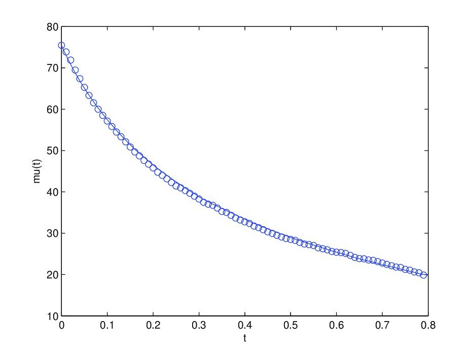 Figure 1
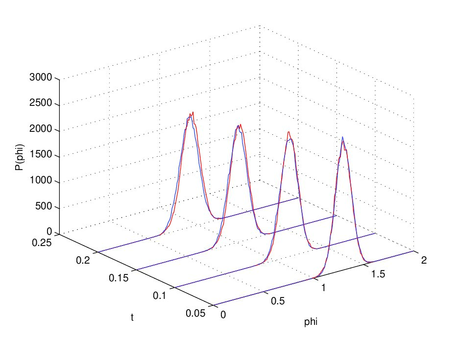 Figure 2
Peer Reviews
No public reviews on file for this paper yet. If you reviewed it on a platform where reviews are public (OpenReview, ICLR, NeurIPS, ICML), you can paste yours below so the community can read it here.
Videos
No videos yet. Explain this paper in a talk, walkthrough, or lecture? Add one.
Equation-Free Implementation of Statistical Moment Closures
Francis J. Alexander and Gregory Johnson
Los Alamos National Laboratory, P.O.Box 1663,
Los Alamos, NM, 87545.
Gregory L. Eyink
Department of Mathematical Sciences
*Johns Hopkins University
Baltimore, MD 21218*
Ioannis G. Kevrekidis
Department of Chemical Engineering and PACM
Princeton University
Princeton, NJ 08544
Abstract
We present a general numerical scheme for the practical implementation of statistical moment closures suitable for modeling complex, large-scale, nonlinear systems. Building on recently developed equation-free methods, this approach numerically integrates the closure dynamics, the equations of which may not even be available in closed form. Although closure dynamics introduce statistical assumptions of unknown validity, they can have significant computational advantages as they typically have fewer degrees of freedom and may be much less stiff than the original detailed model. The closure method can in principle be applied to a wide class of nonlinear problems, including strongly-coupled systems (either deterministic or stochastic) for which there may be no scale separation. We demonstrate the equation-free approach for implementing entropy-based Eyink-Levermore closures on a nonlinear stochastic partial differential equation.
I Introduction
Accurate, fast simulations of complex, large-scale, nonlinear systems remain a challenge for computational science and engineering, despite extraordinary advances in computing power. Examples range from molecular dynamics simulations of proteins MDProteinsI , MDProteinsII and glasses MDGlasses , to stochastic simulations of cellular biochemistry Gillespie ; Wilkinson , to global-scale, geophysical fluid dynamics MajdaWang . Often for the systems under consideration there is no obvious scale separation, and their many degrees of freedom are strongly coupled. The complex and multiscale nature of these processes therefore makes them extremely difficult to model numerically. To make matters worse, one is often interested not in a single, time-dependent solution of the equations governing these processes, but rather in ensembles of solutions consisting of multiple realizations (e.g., sampling noise, initial conditions, and/or uncertain parameters). Often real-time answers are needed (e.g., for control, tracking, filtering). These demands can easily exceed the computational resources available not only now but also for the foreseeable future.
In principle, all statistical information for the problem under investigation is contained in solutions to the Liouville (if deterministic)/Kolmogorov (if stochastic) equations. These are partial differential equations in a state space of high (possibly infinite) dimension. A straightforward discretization of the Liouville / Kolmogorov equations is therefore impractical. An ensemble approach to solving these equations can be taken; however, quite often, the practical application of the ensemble approach is also problematic. Generating a sufficient number of independent samples for statistical convergence can be a challenge. For some problems, computing even one realization may be prohibitive.
The traditional approach to making these problems computationally tractable is to replace the Liouville/Kolmogorov equation by a (small) set of equations (PDEs or ODEs) for a few, low order statistical moments of its solution. When taking this approach for nonlinear systems, one must make an approximation, a closure, for the dependence of higher order moments on lower order moments. Typically the form of the closure equation is based on expert knowledge, empirical data, and/or physical insight. For example, in the superposition approximation and its extensions Superposition for dense liquids and plasmas, both quantum or classical, one approximates third order moments as functions of second order moments. Moment closure methods of this type have been applied to a number of areas including fluid turbulence (see TurbClosure and references therein, and also the work of Chorin et. al.). Of course, as with any approximation strategy, the quality of the resulting reduced description depends on the approximations made – poor closures lead to poor answers/predictions. In addition to replacing the ensemble with a small set of equations for low order moments, these equations are typically easier to solve. They are deterministic and generally far less stiff than the original equations.
A less exploited variant of this approximation scheme is the probability density function (PDF) based moment-closure approach. For PDF moment closures one makes an ansatz for the system statistics guided by available information (e.g., symmetries). One then uses this ansatz in conjunction with the original dynamical equations to derive moment equations. Such PDF-based closures have been developed for reacting scalars advected by turbulence CCK , phase-ordering dynamics Oono and a variety of other systems. This approach to moment-closure is a close analogue of the Rayleigh-Ritz method frequently used in solving the quantum-mechanical Schroedinger equation, by exploiting an ansatz for the wave-function. For a formal development of this point of view, see Eyink96 .
One of the obstacles to applying moment closures is that often the closure equations are too complicated to write down explicitly, even with the availability of computer algebra / symbolic computation systems. This is especially true for large-scale, complex systems, e.g. global climate models. Because of their great complexity, even if one could in principle derive the closure equations analytically, this procedure would be extremely difficult and time-intensive. Moreover, each time a model is updated, as climate and ocean models regularly are, the closure equations would have to be rederived. In other cases it may simply be impossible to determine the closure equations analytically. This is especially likely when PDF’s are not Gaussian, which is the case for most useful closures. Monte Carlo or other numerical methods may be needed in order to evaluate integrals for the moments Levermore96 . In addition, there may be situations where neither analytic nor numerical/MC integration will yield the closure equations due to the black-box nature of the available numerical simulator such as a compiled numerical code with an inaccessible source. Clearly, a need exists for a robust approach to the general closure protocol which circumvents analytical difficulties.
We address that need here by combining PDF closures with equation free modeling EQNFREE EqnFree2 . The basic premise of the equation-free method is to use an ensemble of short bursts of simulation of the original dynamical system to estimate, on demand, the time-evolution of the the closure equations that we may not explicitly have. The equation-free approach extends the applicability of statistical closures beyond the rare cases where they can be expressed in closed form. This hybrid strategy may be faster than the brute-force solution of a large ensemble of realizations of the dynamical equations since the closure version is generally smoother than the original problem.
This paper is organized as follows. In Section 2 we describe the general features of PDF-based moment closures. In Section 3 we explain how to implement the equation-free approach with these closures. We then, in Section 4, apply these ideas for a specific dynamical system, the stochastic Ginzburg-Landau (GL) equations using a particular PDF-based closure scheme, the entropy method of Eyink and Levermore EL . We conclude with a discussion of closure quality, computational issues, and the application of our approach to large-scale systems.
II PDF-Based Moment Closures
We consider the very general class of dynamical systems, including maps, formally represented by
[TABLE]
or
[TABLE]
where is a stochastic process with prescribed statistics. The stochastic component arises from unknown parameters, random forcing, neglected degrees of freedom and/or random initial conditions. This class includes both deterministic and stochastic systems with discrete and/or continuous states. Queueing systems, molecular dynamics, and stochastic PDEs are just some of the many examples that fall into this category.
For concreteness in this paper we restrict ourselves to a special case of equation (2), namely, situations where is a Markov process (Brownian motion, Poisson process, etc.) and—more specifically still—Itô stochastic differential equations of the form:
[TABLE]
The deterministic component of the state, , is governed by the continuously differentiable vector field, . For many problems of interest (e.g., climate) is a highly nonlinear function. The noise component is modeled by the standard mean [math], covariance matrix Wiener process, , possibly modulated by a state-dependent matrix . Equation (3) encompasses a wide class of systems including deterministic ones.
In many cases one is interested in knowing the low order statistics of equation (3), for example an instantaneous mean value or possibly multi-point covariance of . These statistics can be obtained by averaging over an ensemble of stochastic systems, solving equation (3). They can also be obtained via the forward Kolmogorov equation for the probability density function :
[TABLE]
where satisfies the conditions: , and , and where is the generator of the Markov process. In the case of equation (3) this operator takes the form
[TABLE]
The forward Kolmogorov equation then becomes a Fokker-Planck equation
[TABLE]
where is the nonnegative-definite diffusion matrix arising from the noise term. Unlike the original dynamical equation (3), the forward Kolmorogov equation (FKE) is both linear and deterministic. Dealing with it, therefore, has apparent advantages over the original ensemble of stochastic systems simulations. The price to pay for these advantages is that the FKE lives in a typically high, potentially infinite-dimensional, space. When equation (3) is a nonlinear PDE, numerical solution to the FKE is usually ruled out.
For computational purposes, we would therefore like to reduce the FKE (if possible and useful) to a small system of ordinary differential equations. This reduction should simplify the computation as much as possible while retaining fidelity to the original dynamical processes. The reduction proceeds by taking moments of the FKE with respect to a vector-valued function {\mbox{\boldmath\xi}}({\bf X},t) from . The selected should include the relevant variables in the system (slow modes, conserved quantities, etc.). The moments {\mbox{\boldmath\mu}}(t) of {\mbox{\boldmath\xi}}({\bf X},t) are defined by
[TABLE]
and give rise to
[TABLE]
where
[TABLE]
and is the adjoint of or the backward Kolmogorov operator. The result (8) can be obtained by averaging over an ensemble of realizations of the stochastic dynamics (3). In general, however, (8) is not a closed equation for the moments, . One can close this equation by choosing a PDF, P({\bf X},t,{{\mbox{\boldmath\mu}}}), which itself is a function of the moments .
[TABLE]
Alternatively, one can select a family of probability densities P({\bf X},t,{\mbox{\boldmath\alpha}}), specified by parameters {\mbox{\boldmath\alpha}}={\mbox{\boldmath\alpha}}({\mbox{\boldmath\mu}},t) rather than directly by the moments . This is analogous to specifying the temperature in the canonical ensemble as opposed to the average energy. The equivalence of these approaches is guaranteed provided that the parameters and moments can be determined uniquely from one another. The translation between the parameters and their corresponding moments can be carried out by one of several methods. In some cases one may require Monte Carlo evaluation of the resulting integrals.
If the moments and/or parameters are selected judiciously, one hopes that the approximate PDF P({\bf X},t,{\mbox{\boldmath\alpha}}({\mbox{\boldmath\mu}})(t)) will be close to the exact solution of the Liouville/Kolmogorov equation (4). The mapping closure approach of Chen et al CCK and the Gaussian mapping method of Yeung et al. Oono are based on this type of parametric PDF closure 111In the case of CCK the dynamics is an advection-reaction-diffusion equation for a scalar concentration field . The moment functions are the “fine-grained PDF” labelled by space point and scalar value The moment average is the 1-point PDF which gives the distribution of scalar values at space-time point The parametric model P[{\bf X};{\mbox{\boldmath\alpha}},t] is the distribution over scalar fields obtained by the ansatz where is a reference random field of known (Gaussian) statistics and is a “mapping function”. The latter function is the “parameter” which determines (and is determined by) the “moment” from the relation Here is the 1-point PDF of the reference Gaussian field
The approach of Oono is similar. The problem is phase-ordering dynamics as given, for example, by our equation (12) and The moment functions are the quadratic products \xi_{\bf r}[{\bf X},t]=\phi({\bf r},t)\phi({\mbox{\boldmath0}},t), labelled by the displacement and the moment averages are the spatial correlation function . The parametric model P[{\bf X};{\mbox{\boldmath\alpha}},t] is the distribution obtained by the ansatz where is a homogeneous Gaussian random field with mean zero and covariance G({\bf r},t)=\langle u({\bf r},t)u({\mbox{\boldmath0}},t)\rangle and is the stationary planar interface solution of the TDGL equation (12). In this case, it is the auxiliary correlation function which plays the role of the “parameter” It is shown in Oono for various cases how this function may be uniquely related to the “moment” . In fact, perhaps the most familiar application of the parametric approach is the use of the Rayleigh-Ritz method in quantum mechanical calculations. This is the essential approach of our paper.
III Equation-Free Computation
Although we now have obtained a closed moment equation (equation 10), we still need to determine the dynamical vector field . As explained above, this step can be a serious obstacle to the practical implementation of PDF-based moment-closure (PDFMC). A method to calculate is desirable that (i) does not require a radical revision each time the underlying code or model changes, and (ii) is relatively insensitive to the complexity of the PDFMC. The equation-free approach of Kevrekidis and collaborators EQNFREE meets those requirements. It permits one to work with much more sophisticated, physically realistic closures.
Equation-free computation is motivated by the simple observation that numerical computations involving the closure equations ultimately do not require closed formulae for the closure equations. Instead, one must only be able to sample an ensemble of system states distributed according to the closure ansatz P({\bf X},t;{\mbox{\boldmath\alpha}}) and then evolve each of these via equation (3) for short intervals of time. Such sampling and subsequent dynamical evolution would be necessary to calculate the statistics of interest even when not using a closure strategy. It is sufficient to have a (possibly black-box) subroutine available which, given a specific state variable as input, returns the value of the state after a short time . The ensemble of systems, each of which satisfies equation (3), is evolved over a time interval . The moments/parameters or are determined at the beginning and end of this interval and the time derivative {\dot{{\mbox{\boldmath\mu}}}} is estimated from the results of these short ensemble runs. This “coarse timestepper” can be used to estimate locally the right hand side of the closure evolution equations, namely {\bf V}({{\mbox{\boldmath\mu}}},t).
Coarse projective forward Euler (arguably the simplest of equation-free algorithms) which we will use below illustrates the approach succinctly: Starting from a set of coarse-grained initial conditions specified by moments {\mbox{\boldmath\mu}}(t) we first (a) lift to a consistent fine scale description, that is, sample the PDF ansatz P({\bf X},t;{\mbox{\boldmath\alpha}}(t)) to generate ensembles of initial conditions for equation (3) consistent with the set {\mbox{\boldmath\mu}}(t); (b) starting with these consistent initial conditions we evolve the fine scale description for a (relatively short) time ; we subsequently restrict back to coarse observables by evaluating the moments {\mbox{\boldmath\mu}}(t+\delta t) as ensemble-averages and (d) use the results to estimate locally the time derivative d{\mbox{\boldmath\mu}}/dt. This is precisely the right hand-side of the explicitly unavailable closure, obtained not through a closed form formula, but rather through short, judicious computational experiments with the original fine scale dynamics/code. Given this local estimate of the coarse-grained observable time derivatives, we can now exploit the smoothness of their evolution in time (in the form of Taylor series) and take a single long projective forward Euler step:
[TABLE]
The procedure then repeats itself: lifting, fine scale evolution, restriction, estimation, and then (connecting with continuum traditional numerical analysis) a new forward Euler step. Beyond coarse projective forward Euler, many other coarse initial-value solvers (e.g. coarse projective Adams-Bashforth, and even implicit coarse solvers) have been implemented; the stability and accuracy study of such algorithms is progressing EQNFREE . These developments allow us to construct a nonintrusive implementation of PDF moment closures, nonintrusive in the sense that we compute with the closures without explicitly obtaining them, but rather by intelligently chosen computational experiments with the original, fine-scale problem.
There is, however, an obvious objection to the equation-free implementation of moment-closures. Using the same ingredients, one can clearly obtain an estimate of any statistics of interest (for example, the moment-averages {\mbox{\boldmath\mu}}(t)) without the need of making any closure assumptions whatsoever. This can be done by the much simpler method of direct ensemble averaging. That is, one can sample an ensemble of initial conditions from any chosen distribution , evolve each of these realizations according to the fine-scale dynamics of equation (3), and then evaluate any statistics of interest at time by averaging over the ensemble of solutions It would seem that this direct ensemble approach is much more straightforward and accurate than the equation-free implementation of a moment-closure, which introduces additional statistical hypotheses.
The response to this important objection is that the fine-scale dynamics (3) is often very stiff for the applications considered, in which the system contains many-degrees-of-freedom interacting on a huge range of length- and time-scales. In contrast, the closure equation (10) is much less stiff, because of statistical-averaging, and its solutions {\mbox{\boldmath\mu}}(t) are much smoother in time (and space). Thus, to evolve an ensemble of solutions of the fine-scale dynamics (3) from an initial time to a final time would require integration steps, where the time-step is required to be very small by the intrinsic stiffness of the micro-dynamics. In the closure approach, the evolution of the moment equations (10) from time to time requires only integration steps, with (hopefully) Each of these closure integration steps by an increment requires in the equation-free approach just one (or just a few) fine-scale integration step by an increment Thus, there is an over-all savings by a (hopefully) large factor This crude estimate is based on a single step coarse projective forward Euler algorithm; clearly, more sophisticated projective integration algorithms can be used.
In all of them, however, the computational savings are predicated on the smoothness of the closure equations, and are governed by the ratio of the time that it takes to obtain a good local estimate of d{\mbox{\boldmath\mu}}/dt from full direct simulation to the time that we can (linearly or even polynomially) extrapolate {\mbox{\boldmath\mu}}(t) in time. It is also worth noting that a variety of additional computational tasks, beyond projective integration (e.g. accelerated fixed point computation) can be performed within the equation-free framework
In the next section we show by a concrete example how significant computational economy can be achieved with statistical moment closures implemented in the equation-free framework.
IV A Numerical Example
We illustrate here the equation-free implementation of moment-closures for a canonical equation of phase-ordering kinetics Bray , the stochastic time-dependent Ginzburg-Landau (TDGL) equation in one spatial dimension. This is written as
[TABLE]
where represents a local order parameter, e.g. a magnetization. The noise has mean zero and covariance . The potential shall be chosen as
[TABLE]
to represent a single quartic/quadratic well. This stochastic dynamics has an invariant measure which is formally of Hamiltonian form where
[TABLE]
The Gibbsian measure is approached at long times for any random distribution of initial states.
One of the simplest dynamical quantities of interest is the bulk magnetization where is the total volume. If the initial statistics are space-homogeneous, then the ensemble average is also given by for any space point Equation (12) leads to a hierarchy of equations for statistical moments of . For example, the first moment satisfies the equation
[TABLE]
The evolution of the mean total magnetization is thus a function of the mean cubic total magnetization. One could write a time evolution equation for , but it would involve a higher order term , and so on. Each equation contains higher moments and therefore the hierarchy does not close.
To close the equation for we assume a parametric PDF of the form where
[TABLE]
is a perturbation of the Hamiltonian (13) by a term proportional to the moment variable This is a special case of a general “entropy-based” closure prescription proposed by Eyink and Levermore EL . This closure scheme guarantees that at long times and therefore the PDF ansatz relaxes to the correct stationary distribution of the stochastic process. The determination of the parameter given the moment is here accomplished by Legendre transform
[TABLE]
where the “moment-generating function” and denotes average with respect to the invariant measure . The numerical optimization required for the Legendre transform is well-suited to gradient descent algorithms such as the conjugate gradient method, since
[TABLE]
where is the average of the moment-function in the PDF ansatz In simple cases, and may be given by closed analytical expressions. If not, then both of these averages may be determined together by Monte Carlo sampling techniques.
In the numerical calculations below, we discretize equation (12) using a forward Euler-Maruyama stochastic integrator and 3-point stencil for the Laplacian (other discretizations are possible).
[TABLE]
where are independent, identically distributed standard normal random variables for each space-time point The invariant distribution of the stochastic dynamics space-discretized in this manner has a Gibbsian form with discrete Hamiltonian
[TABLE]
where are nearest-neighbor pairs. The closure ansatz can be adopted in the consistently discretized form where
[TABLE]
In this numerical experiment, we integrate an member ensemble of solutions of equation (IV), and measure the ensemble-averaged, global magnetization at each time-step. With this we compare the results of the entropy-based closure simulation implemented by the equation-free framework using also an ensemble with samples. In this concrete example, the projective integration scheme works as follows: Suppose we are given the parameter at time . The mean is first calculated from the parametric ensemble at time by Monte Carlo sampling. Next all samples are integrated over a short time-step to create a time-advanced ensemble. From this ensemble is calculated, which yields an estimate of the local time derivative.
[TABLE]
A large, projective Euler time-step of the moment average is then taken via
[TABLE]
The parameter is finally updated by using the Legendre transform inversion to obtain from the known value The cycle may now be repeated to integrate the closure equations by successive time-steps of length
A critical issue in general application of projective integration is the criterion to determine the projective time-step For stiff problems with time-scale separation, the projective time step for stability purposes is of the order of (1/fastest “slow group” eigenvalues), while the “preparatory” simulation time is of the order of (1/slowest “fast group” eigenvalue). Variants of the approach have been developed for problems with several gaps in their spectrum GK1 . Accuracy considerations in real-time projective step selection can, in principle, be dealt with in the traditional way for integrators with adaptive step-size selection and error control: through on-line a posteriori error estimates. An additional “twist” arises from the error inherent in the estimation of the (unavailable) reduced time derivatives from the ensemble simulations; issues of variance reduction and even on-line hypothesis testing (are the data consistent with a local linear model?) must be considered. These are important research issues that are currently explored by several research groups. Nevertheless, the main factor in computational savings comes from the effective smoothness of the unavailable closed equation: the separation of time scales between the low-order statistics we follow and the higher order statistics whose effect we model (and, eventually, the time scales of the direct simulation of the original model).
Figure 1 is a plot comparing Projective Integration with Entropy Closure and direct Ensemble Integration with equation (12) for diffusion constant We have selected both the “fine-scale” integration step and the “coarse-scale” projective integration step to be as large as possible, consistent with stability and accuracy. Thus, only steps small enough to avoid numerical blow-ups were considered. Then, values were selected both for and for so that the numerical integrations with those time-steps differed by at most a few percent from fully converged integrations with very small steps. In this manner, the time step required for the Euler-Maruyama integration of (12) was determined to be . On the other hand, for projective integration of the closure equation a time step could be taken. This indicates a gain in time step by a factor of 25, which is also roughly the speed-up in the algorithm or savings in CPU time. The present example is not as stiff as equations that appear in more realistic applications, with a very broad range of length- and time-scales, where even greater computational economies might be expected.
In general, the moment-closure results need not agree so well with those of the direct ensemble approach, even when both are converged. In the example presented here, there is good agreement because the closure effectively captures the one-point PDF (see Fig.2). This one-point PDF is the only statistical quantity that enters into Equation (14) as long as the statistics are homogeneous and the Laplacian term vanishes.
V Conclusions
In this paper, we have described how one can combine recently developed equation-free methods with statistical moment closures to model nonlinear problems. With this method we can numerically integrate complex nonlinear systems, for which closure equations may not be available in closed form. In the example presented here the specific entropy-based closure we selected has an H-theorem which guarantees relaxation to the equilibrium state of the original dissipative dynamics. However, we stress that the general approach outlined above can be used with a variety of closure methods.
The equation-free method has the potential to enhance the flexibility, power, and applications set of the statistical moment closure approach. Since little or no analytic work is required, the sophistication of statistical moment closures can greatly enhanced beyond Gaussian PDF ansätze. The “practical usefulness” criterion for parametric PDF models that they permit analytical calculations is replaced by the criterion that they can be efficiently sampled. We believe that this approach can significantly increase the usefulness of closure methods.
In order to model systems like global climate, oceans, and reaction diffusion processes in systems biology, one will have to construct more complex closures. These will likely include higher order moments, correlation functions of the relevant variables, highly non-Gaussian statistics, etc. As the closures become more complex, the lifting step will require more efficient sampling approaches. One will likely have to use nonlocal, accelerated sampling methods. One will also likely employ the latest in adaptive time and adaptive mesh methods to optimize performance for large-scale problems.
VI Acknowledgements
This work, LA-UR-07-2218, was carried out in part at Los Alamos National Laboratory under the auspices of the US National Nuclear Security Administration of the US Department of Energy. It was supported under contract number DE-AC52-06NA25396. The work of IGK was partially supported by DARPA and by and US DOE(CMPD). G. Eyink was supported by NSF-ITR grant, DMS-0113649.
The reference list from the paper itself. Each links out to its DOI / PubMed record.
- 1(1) T. Schlick, R. D. Skeel, A. T. Brunger, L. V. Kale, J. A. Board, Jr. , J. Hermans, and K. Schulten J. Comp. Phys. 151 , 9, (1999).
- 2(2) M. Karplus and J. A. Mc Cammon, Nature, Structural and Molecular Biology , 9 , 646, (2002).
- 3(3) P. G. Debenedetti and F. H. Stillinger, Nature , 410 , 259, (2001).
- 4(4) D. T. Gillespie, J. Phys. Chem. , 81 , 2340, (1977).
- 5(5) D. J. Wilkinson, Stochastic Modeling for Systems Biology , Chapman & Hall / CRC Press, Boca Raton, (2006).
- 6(6) A. J. Majda and X. Wang, Nonlinear Dynamics and Statistical Theories for Basic Geophysical Flows, Cambridge Univeristy Press, Cambridge UK, 2006
- 7(7) J. P. Hansen and I. R. Mac Donald, Theory of Simple Liquids , Academic, New York, (1986).
- 8(8) S. B. Pope, Turbulent Flows , Cambridge University Press, Cambridge, UK, (2000).