Dynamical Casimir effect for gravitons in bouncing braneworlds
Marcus Ruser, Ruth Durrer

TL;DR
This paper investigates the creation of gravitons in a five-dimensional braneworld scenario with bouncing branes, analyzing their spectrum, energy density, and implications for cosmology, including constraints from nucleosynthesis and dark matter considerations.
Contribution
It provides a detailed calculation of graviton production in a bouncing braneworld, highlighting the spectrum, energy density, and the role of Kaluza-Klein modes, with implications for cosmology.
Findings
Massless gravitons have a blue spectrum.
Energy density satisfies nucleosynthesis bounds.
Kaluza-Klein modes unlikely to be dark matter.
Abstract
We consider a two-brane system in a five-dimensional anti-de Sitter spacetime. We study particle creation due to the motion of the physical brane which first approaches the second static brane (contraction) and then recedes from it(expansion). The spectrum and the energy density of the generated gravitons are calculated. We show that the massless gravitons have a blue spectrum and that their energy density satisfies the nucleosynthesis bound with very mild constraints on the parameters. We also show that the Kaluza-Klein modes cannot provide the dark matter in an anti-de-Sitter braneworld. However, for natural choices of parameters, backreaction from the Kaluza-Klein gravitons may well become important. The main findings of this work have been published in the form of a Letter [R. Durrer and M. Ruser, Phys. Rev. Lett. 99, 071601 (2007), arXiv:0704.0756].
Click any figure to enlarge with its caption.
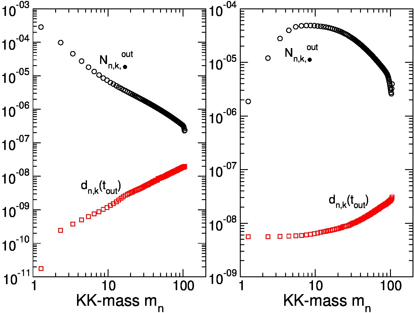 Figure 1
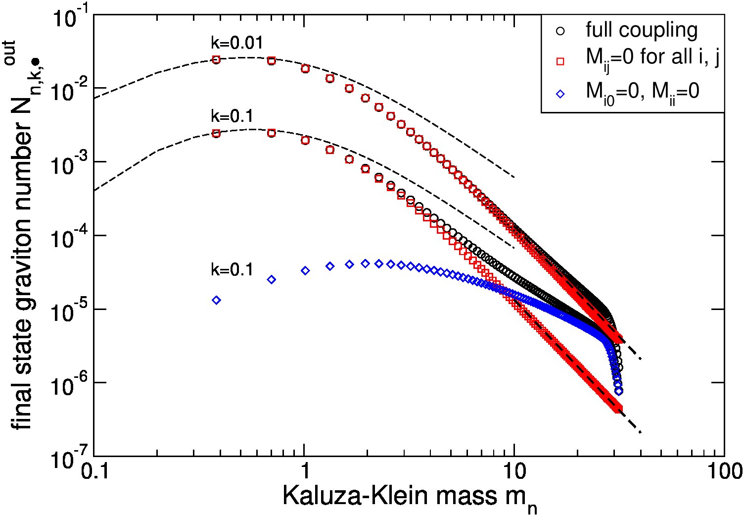 Figure 1
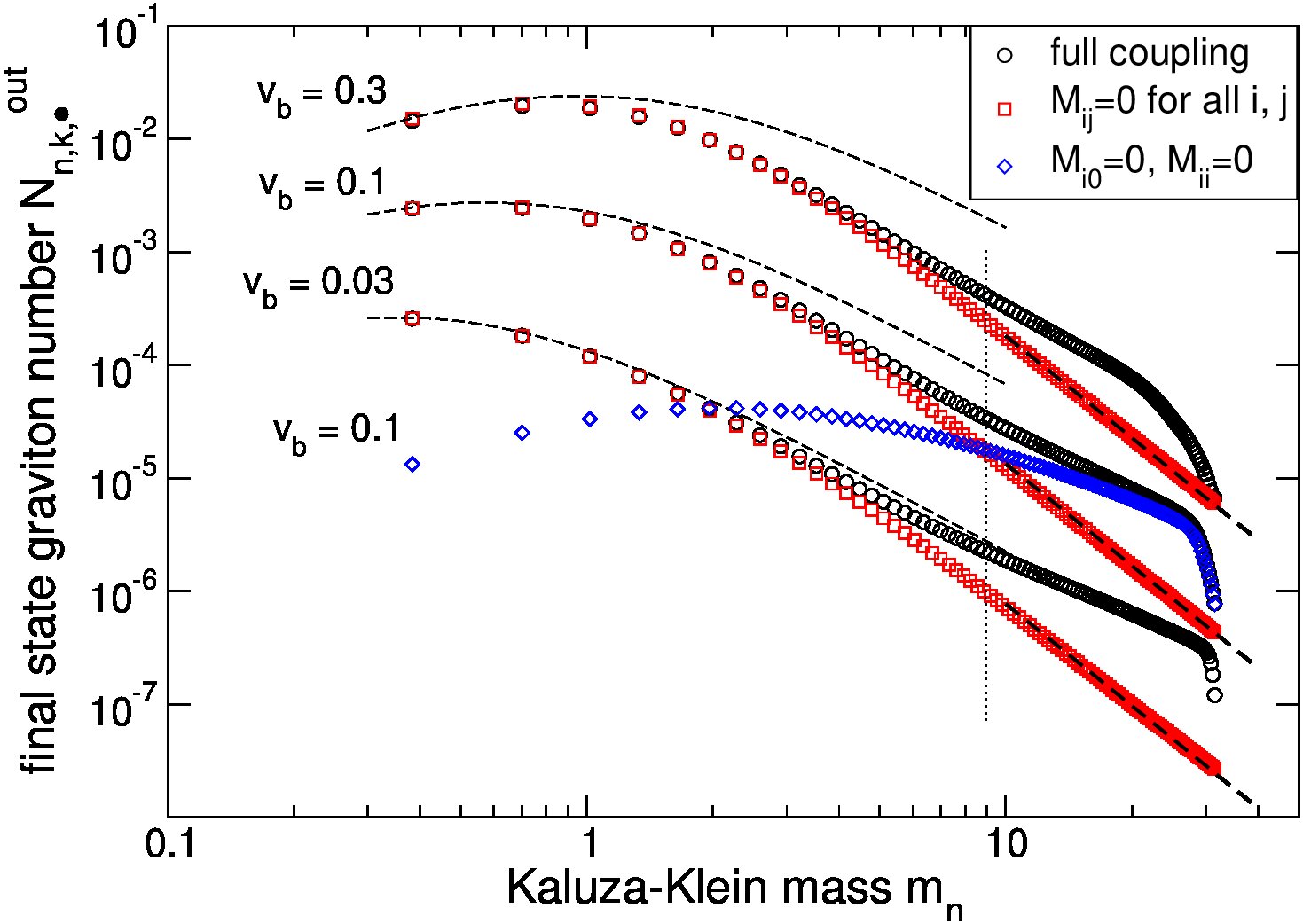 Figure 2
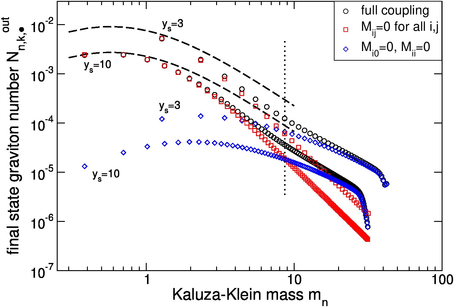 Figure 3
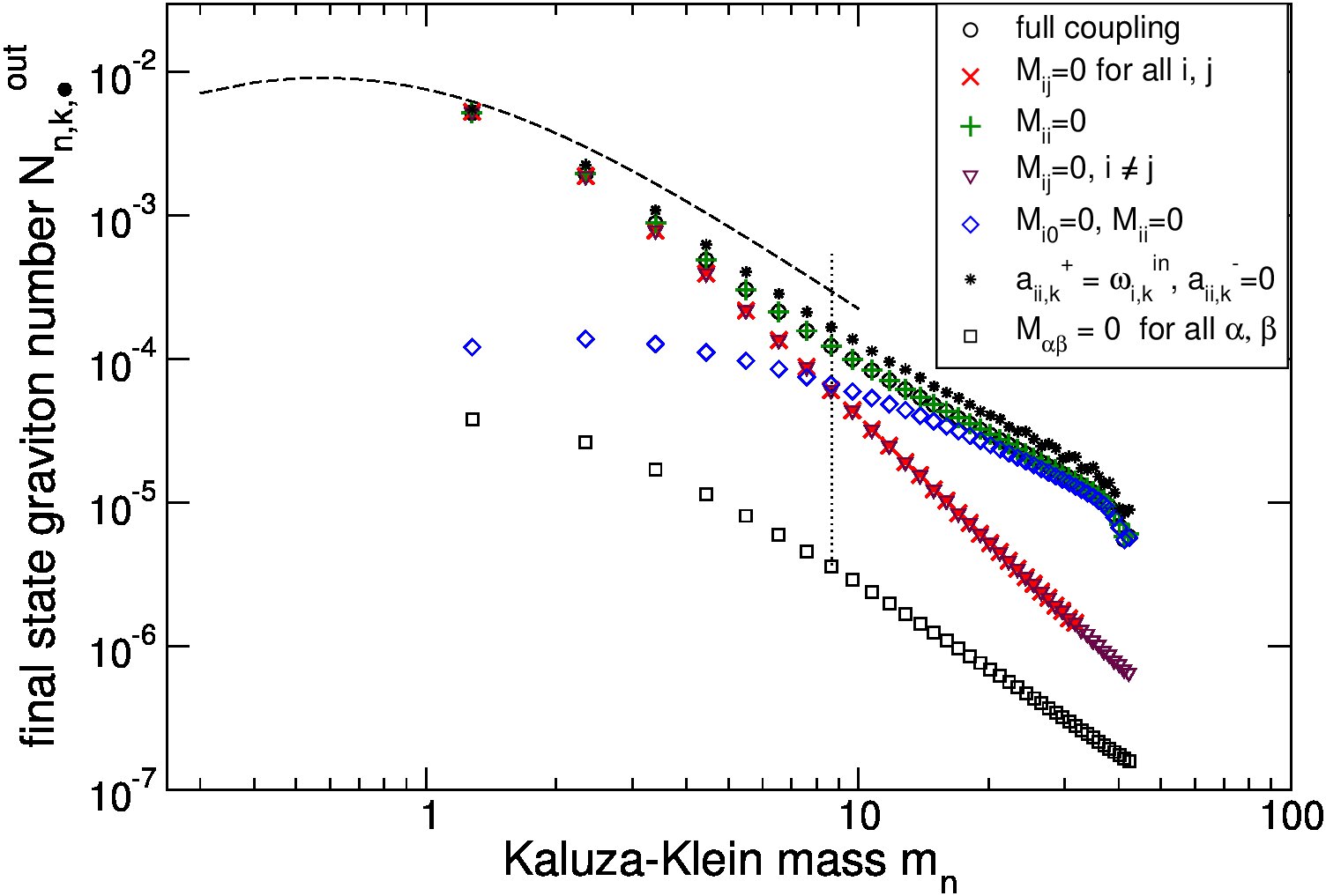 Figure 4
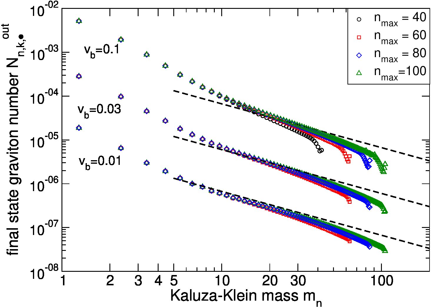 Figure 5
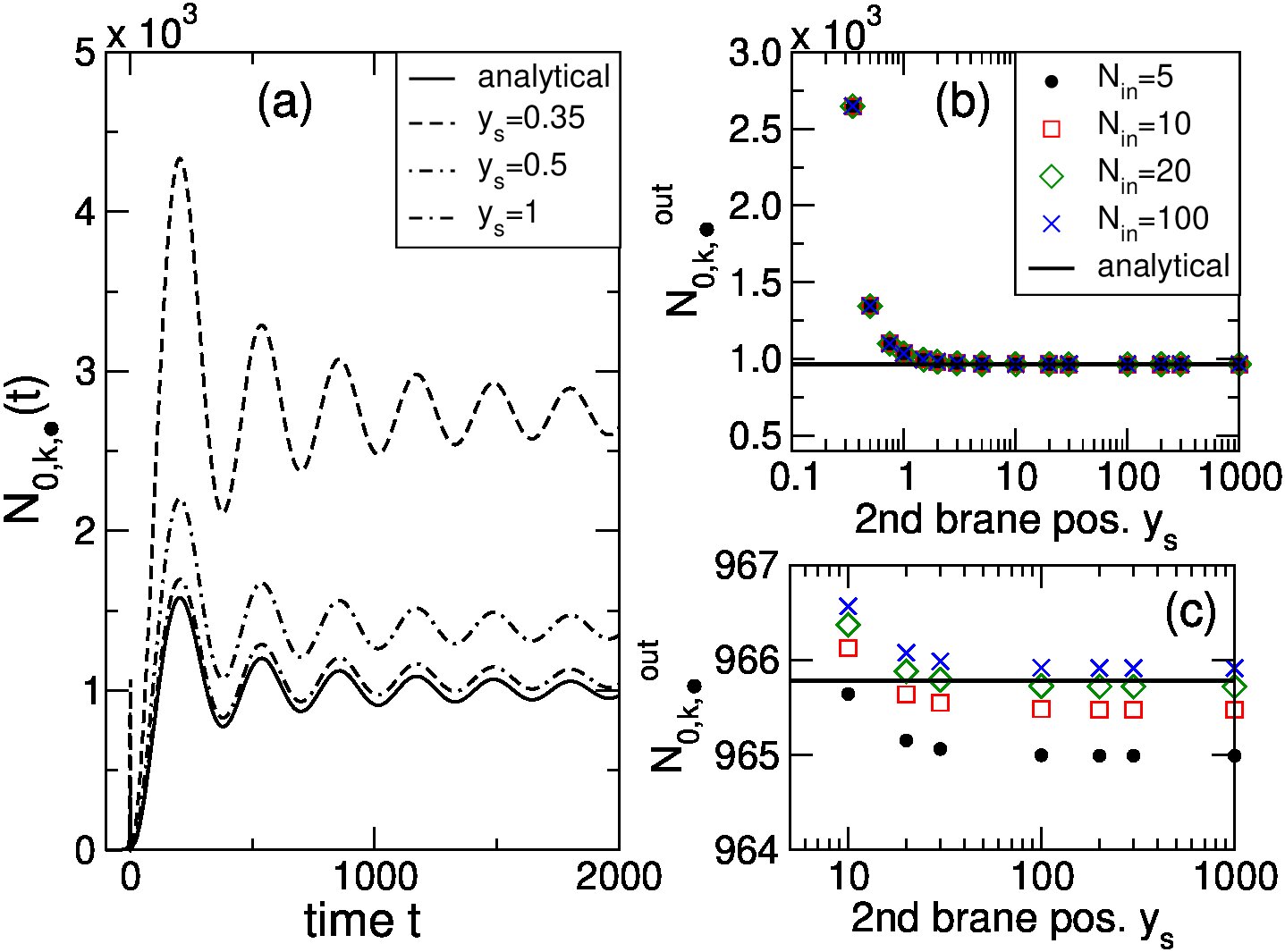 Figure 5
 Figure 2
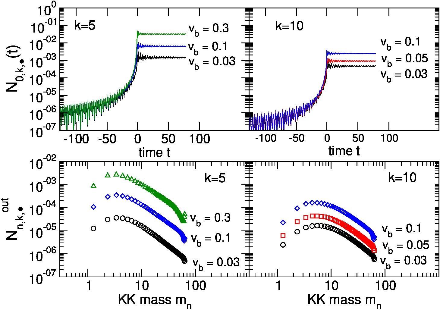 Figure 3
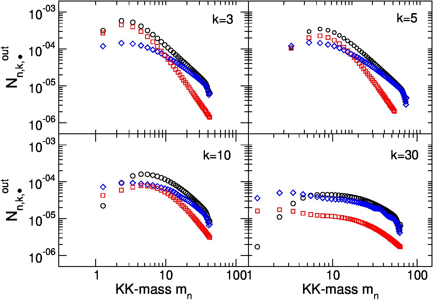 Figure 4
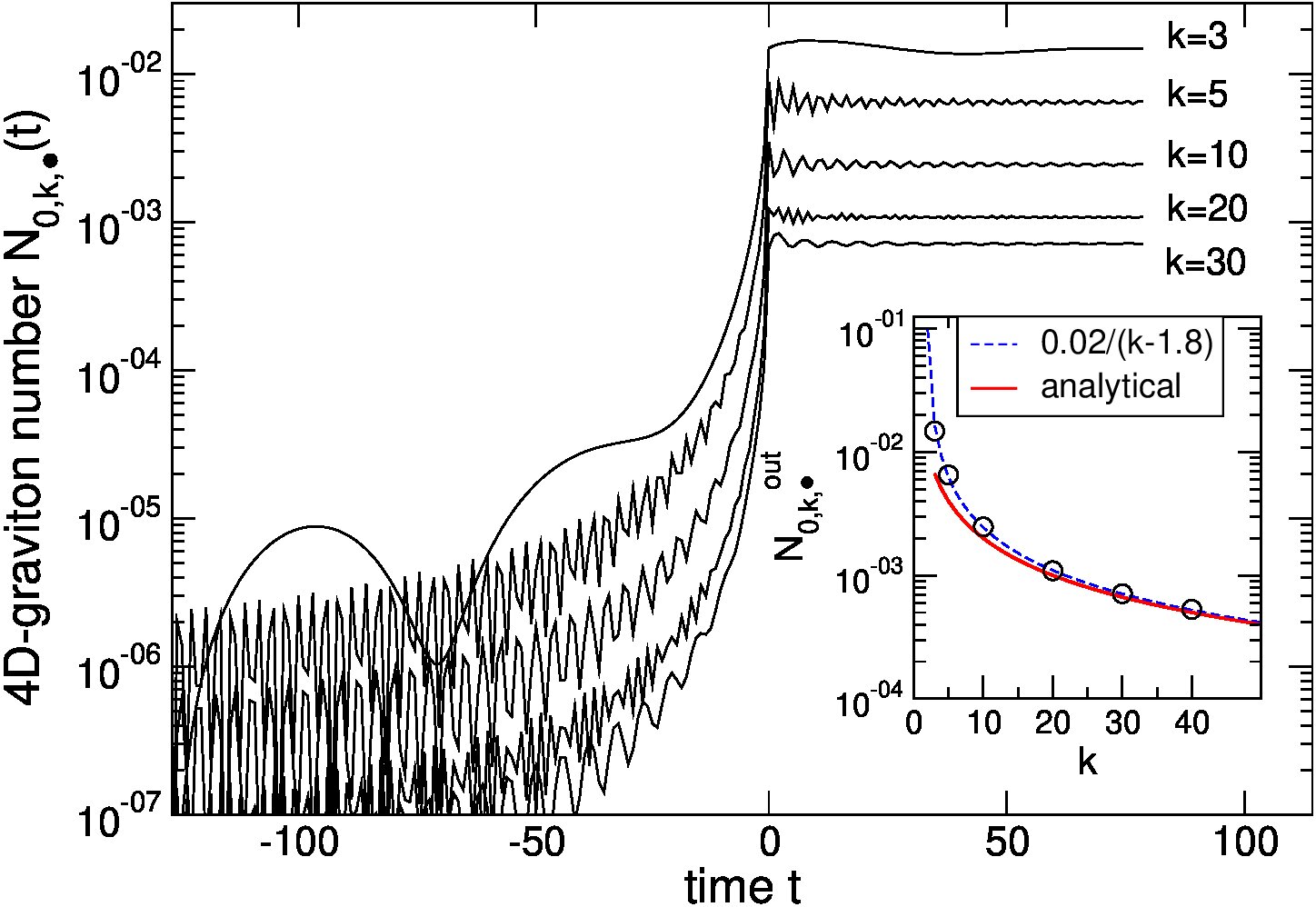 Figure 6
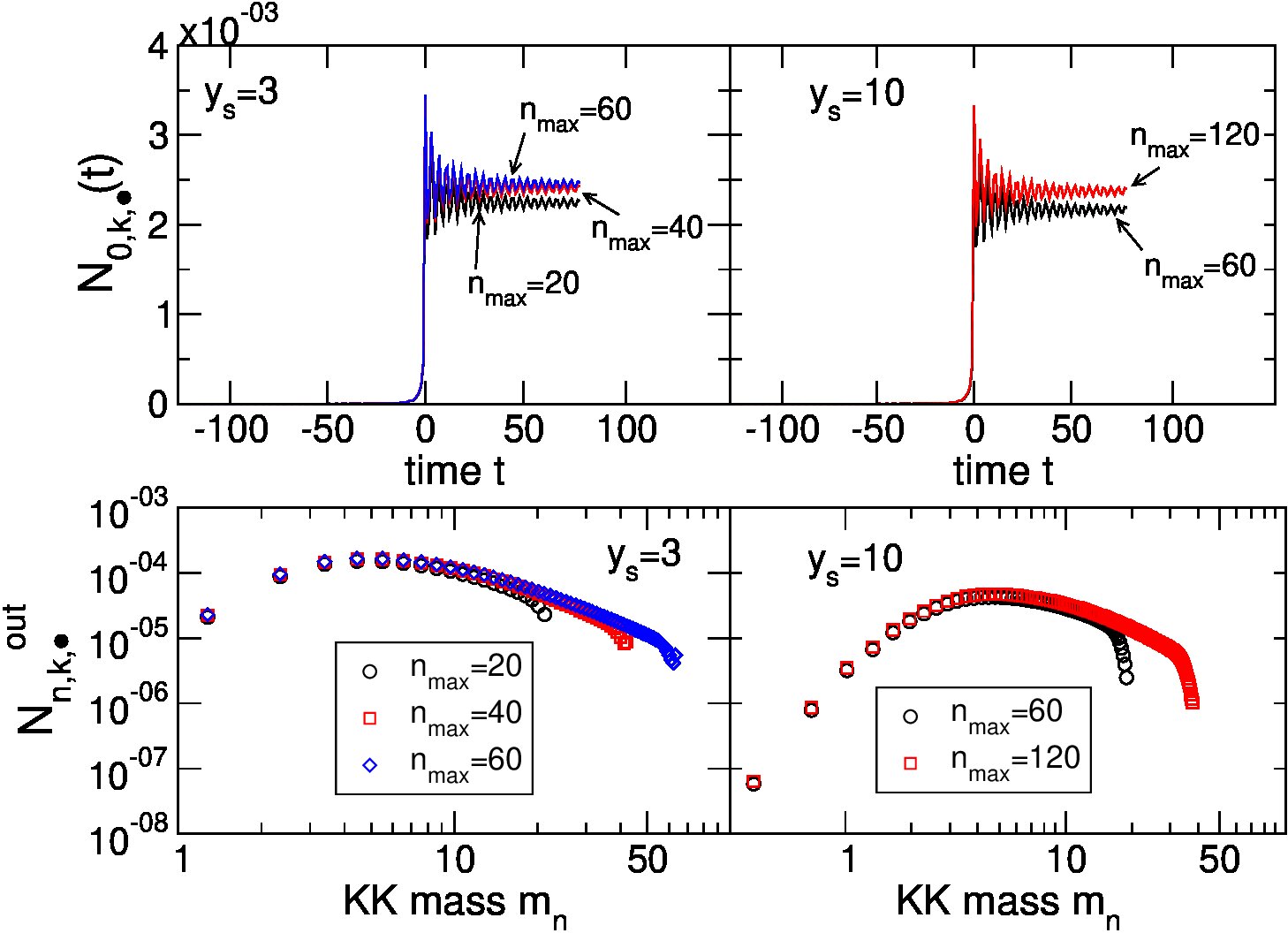 Figure 7
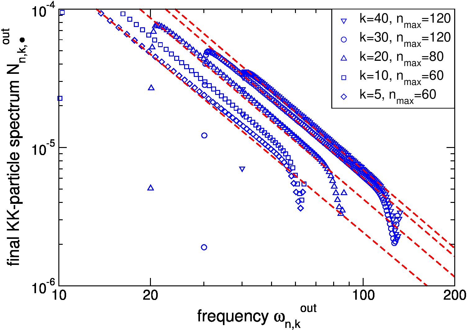 Figure 8
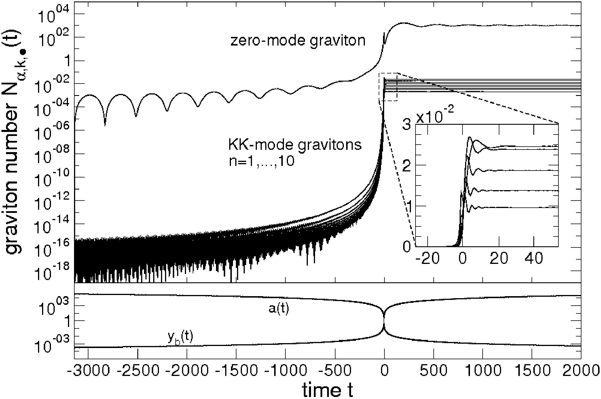 Figure 1
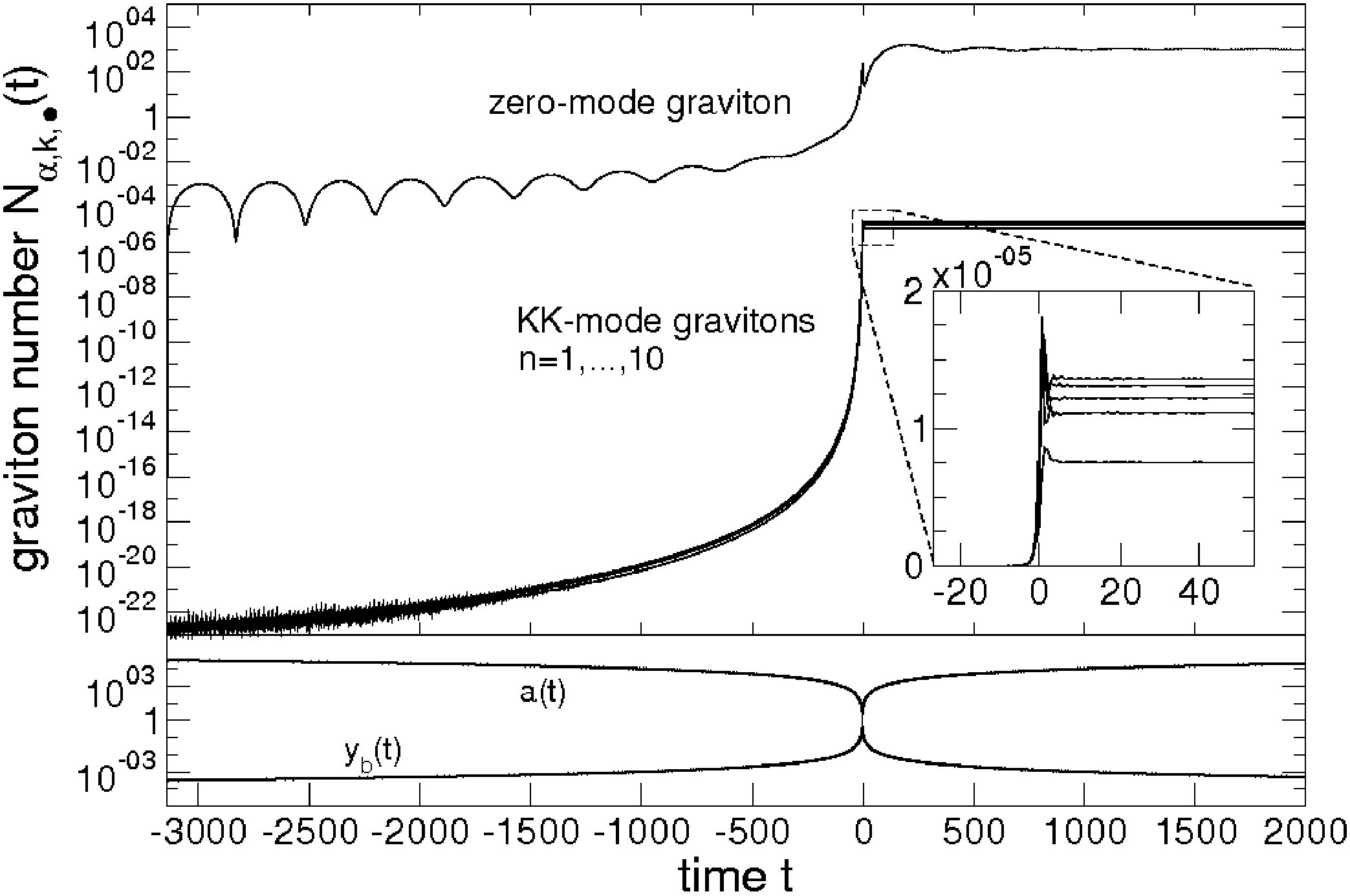 Figure 2
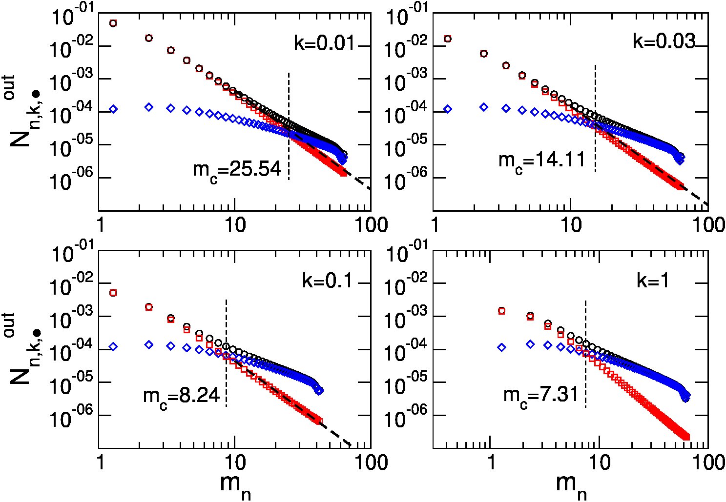 Figure 16
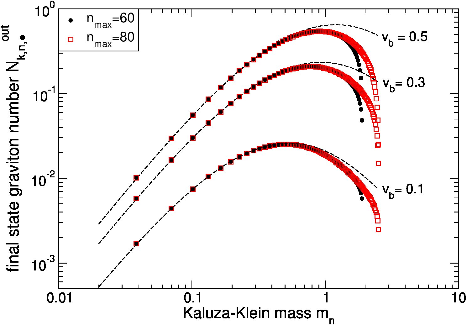 Figure 1
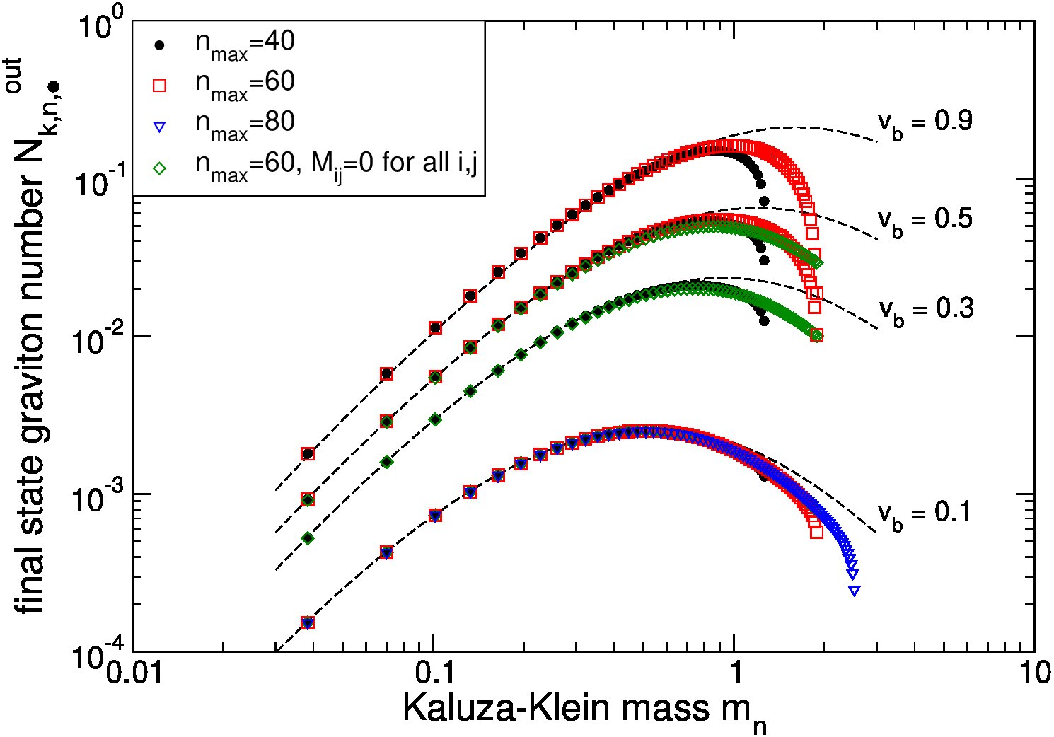 Figure 2
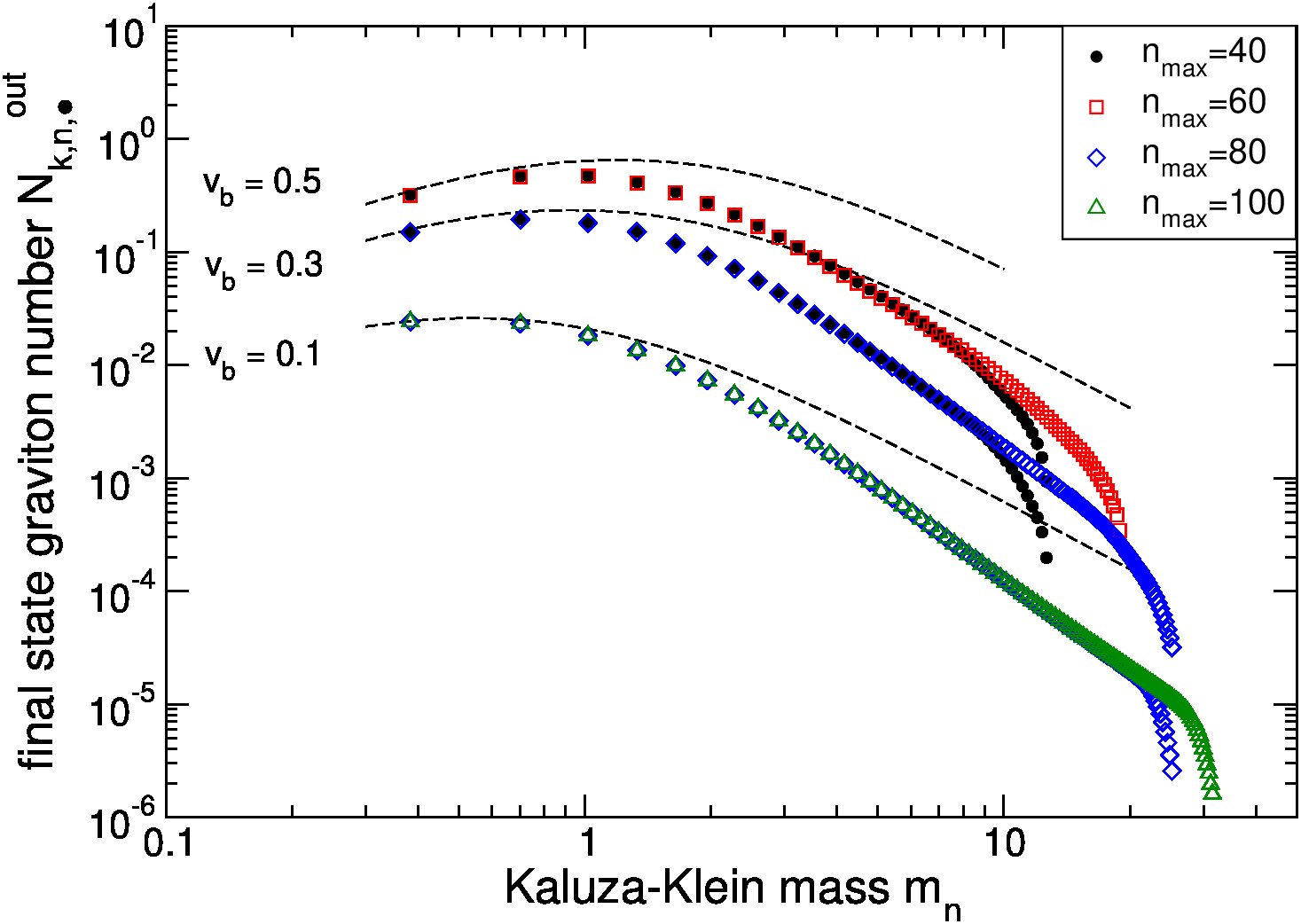 Figure 3
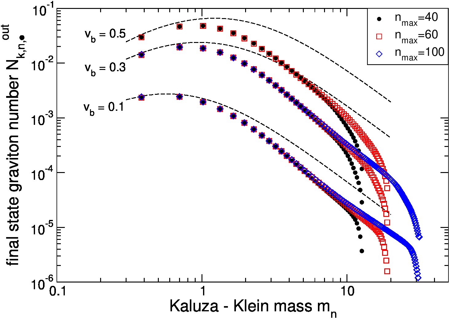 Figure 4
 Figure 21
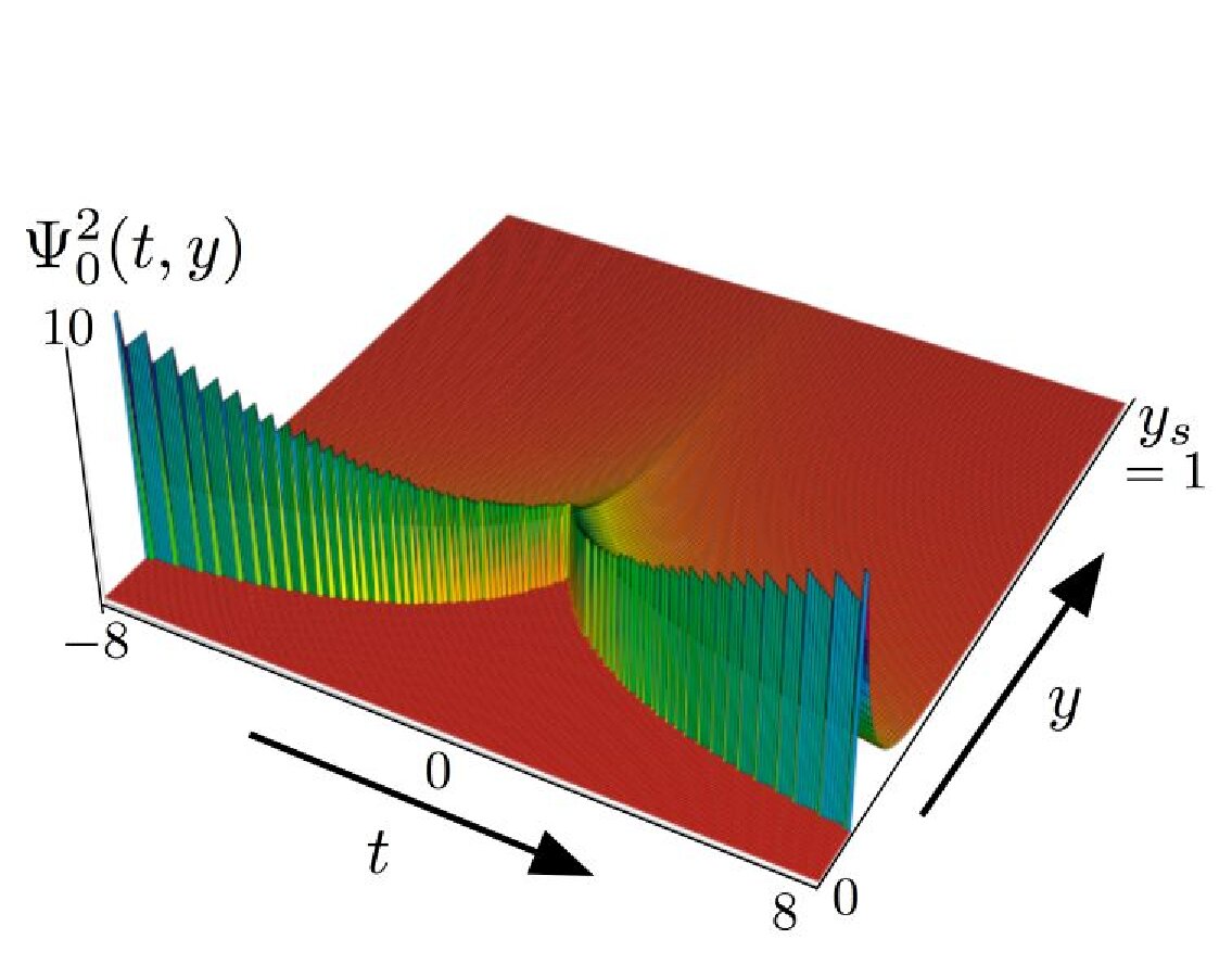 Figure 22
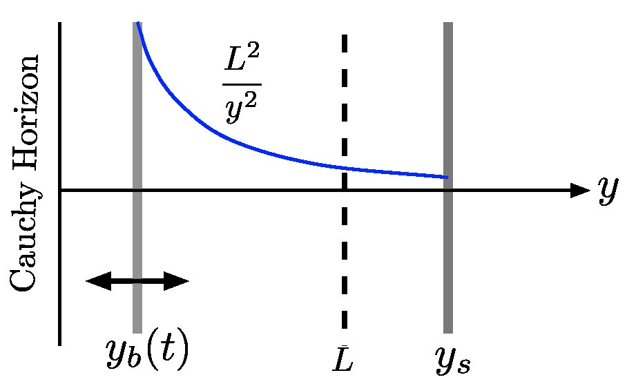 Figure 23
 Figure 3
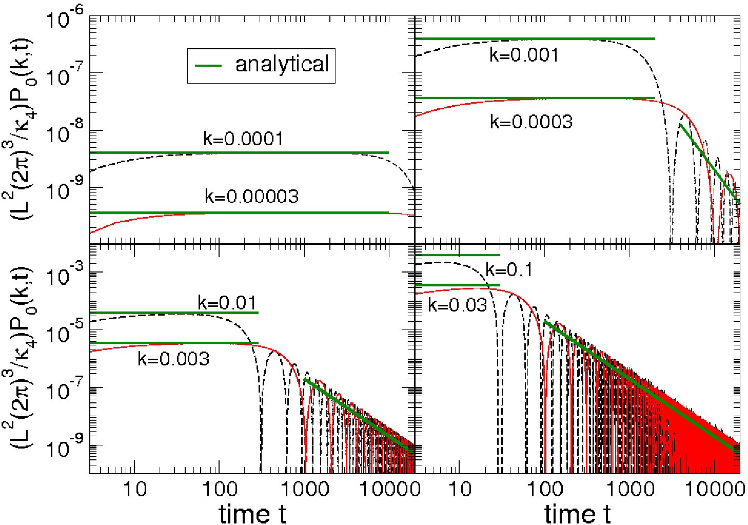 Figure 4
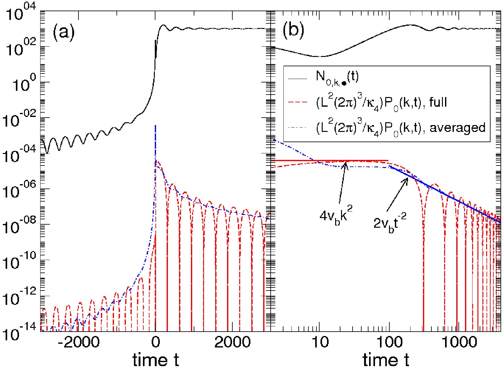 Figure 26
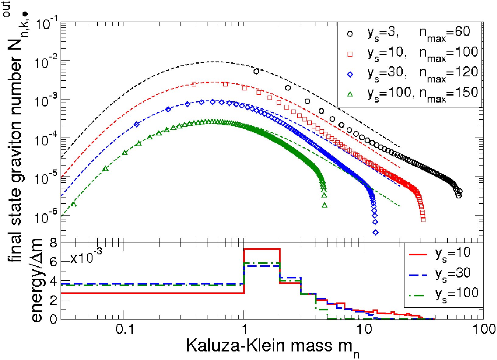 Figure 27
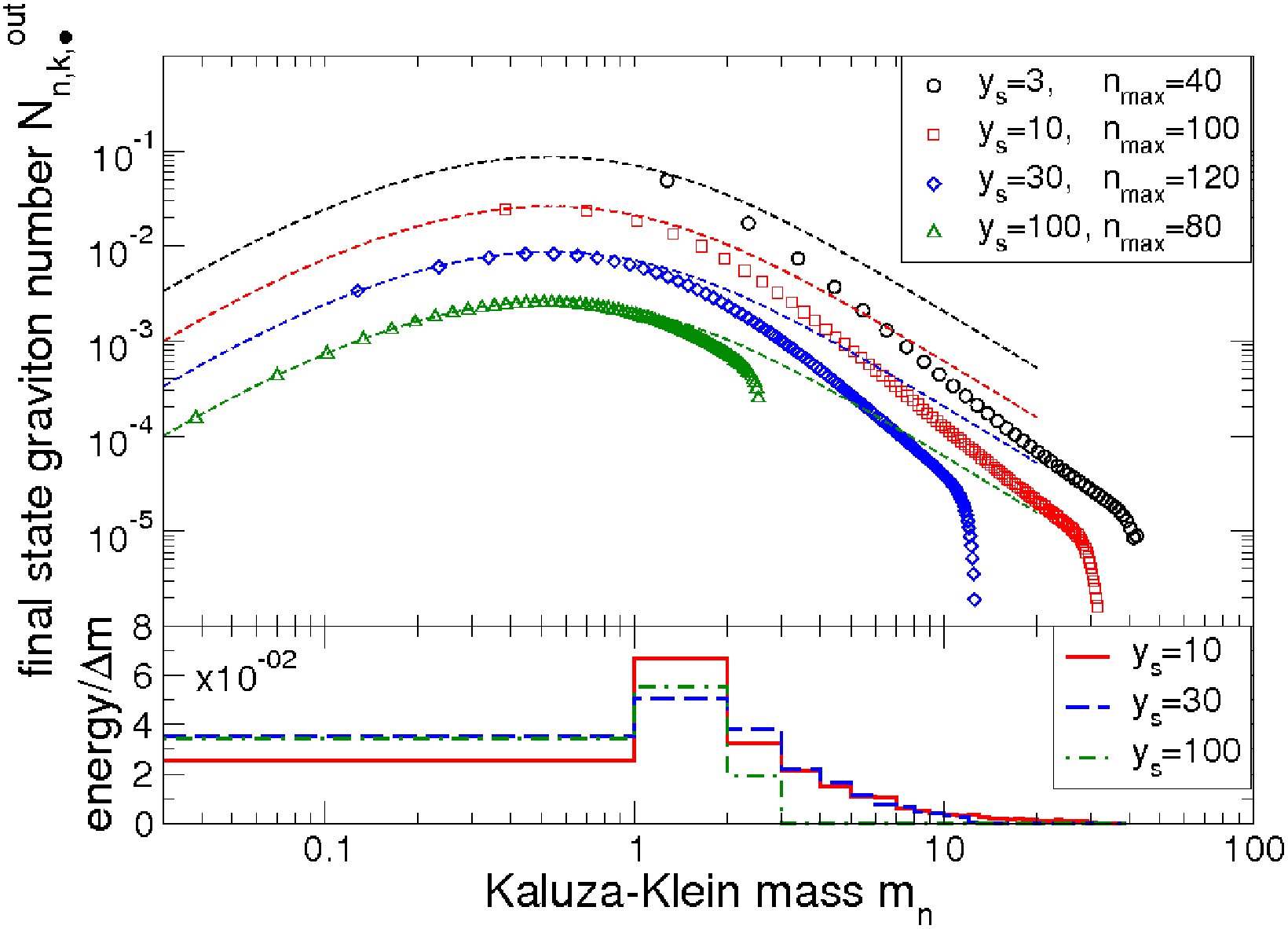 Figure 28
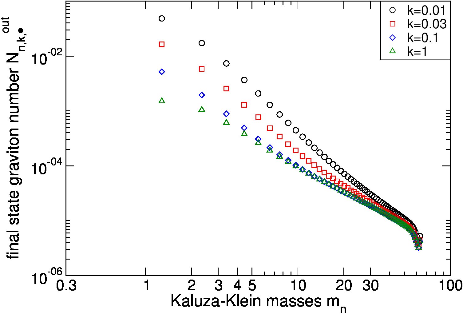 Figure 29
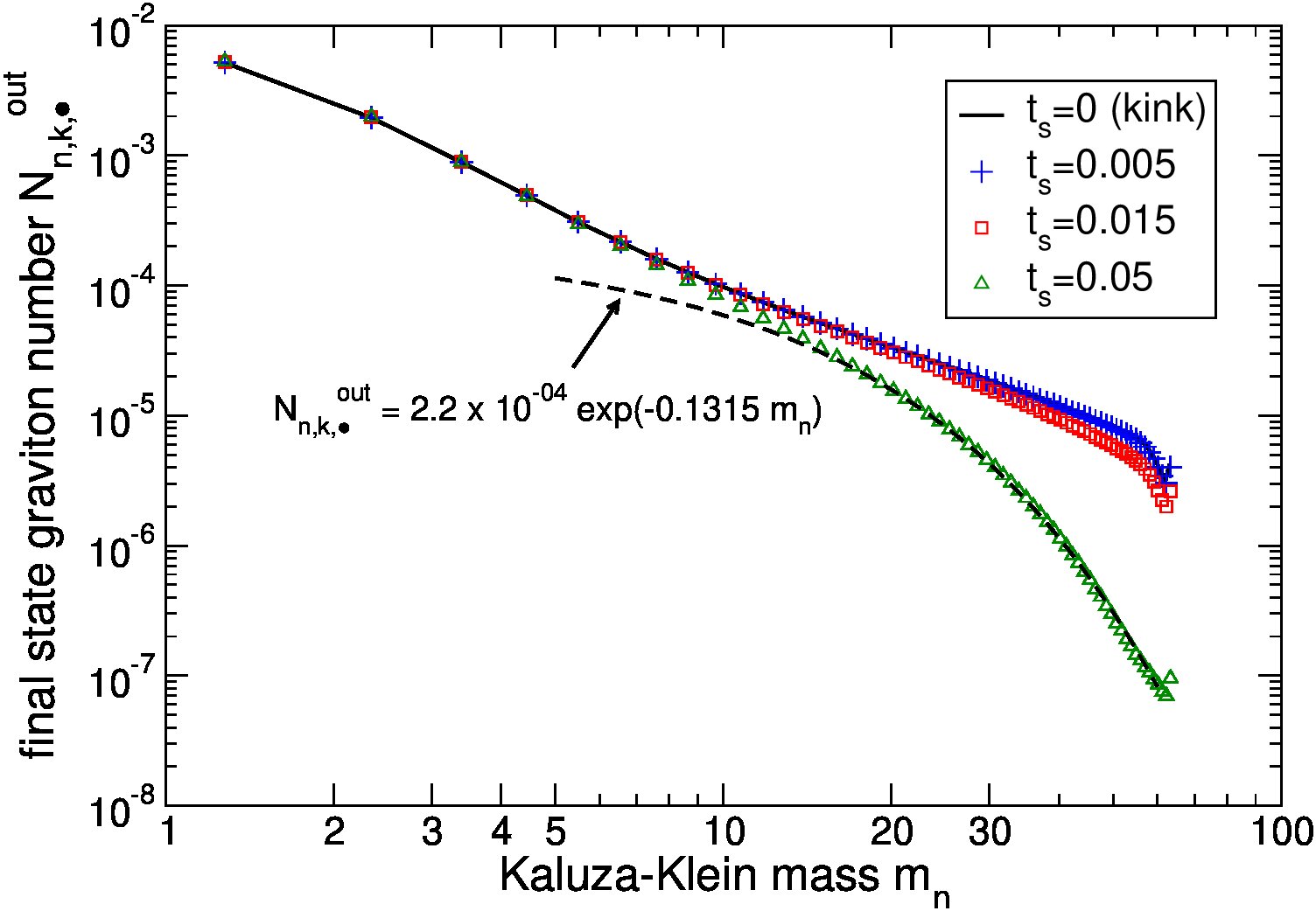 Figure 30
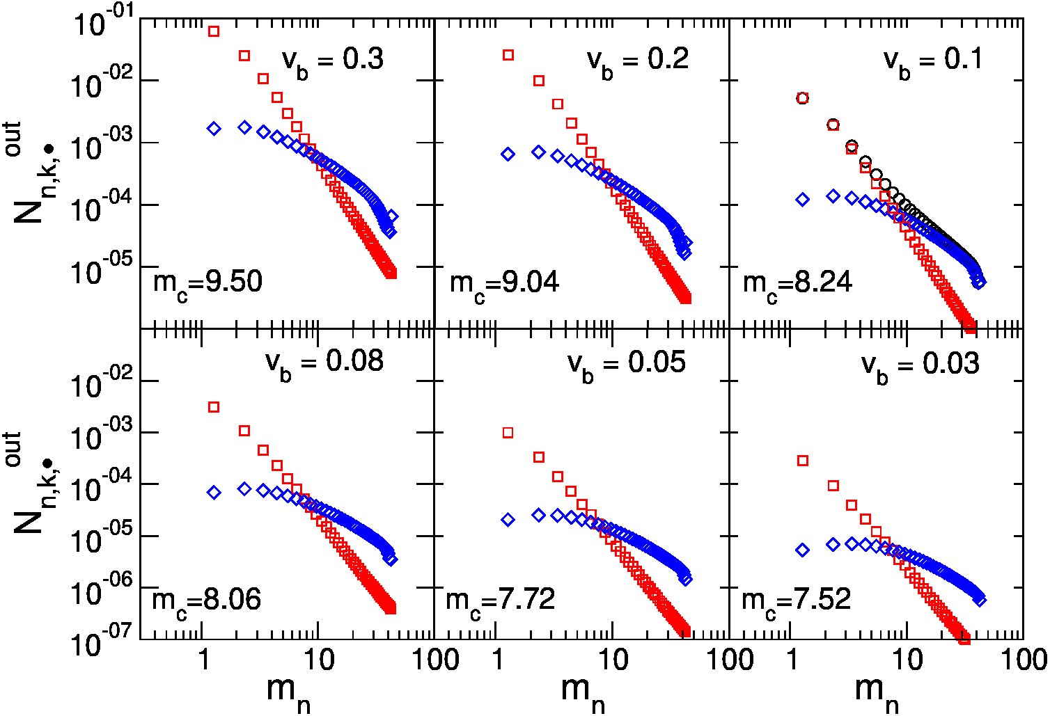 Figure 31
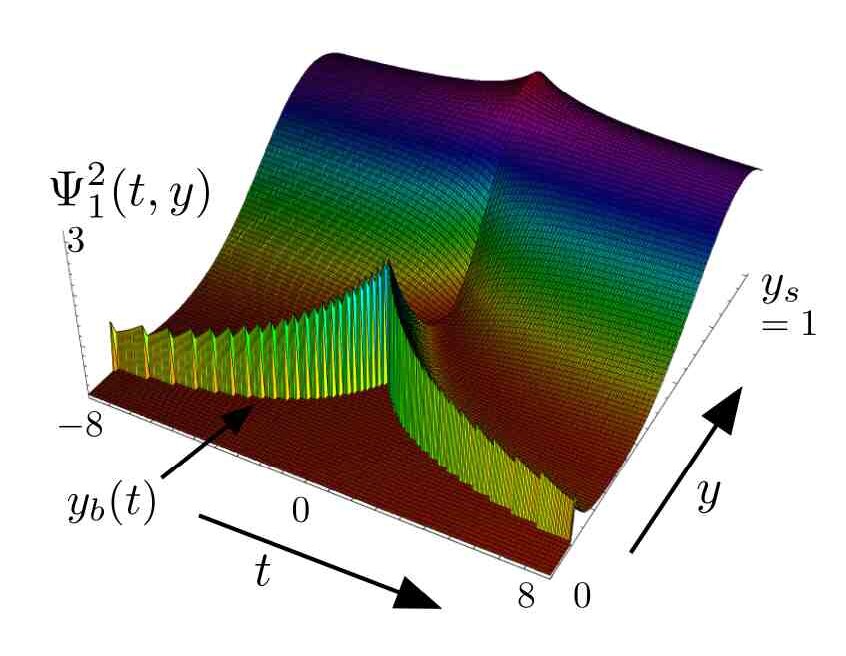 Figure 32
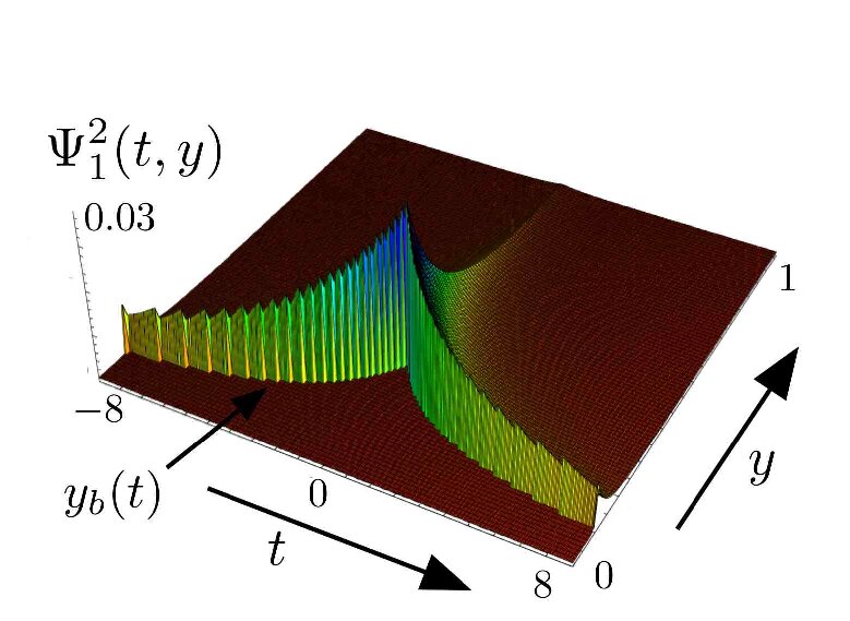 Figure 33
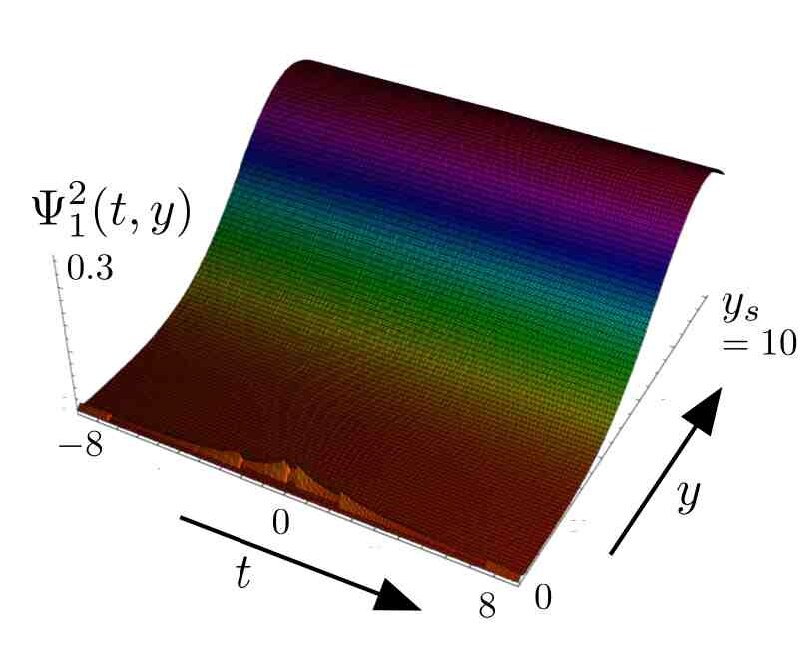 Figure 34
Peer Reviews
No public reviews on file for this paper yet. If you reviewed it on a platform where reviews are public (OpenReview, ICLR, NeurIPS, ICML), you can paste yours below so the community can read it here.
Videos
No videos yet. Explain this paper in a talk, walkthrough, or lecture? Add one.
Dynamical Casimir effect for gravitons in bouncing braneworlds
Marcus Ruser
Ruth Durrer
Département de Physique Théorique, Université de Genève, 24 quai Ernest Ansermet, 1211 Genève 4, Switzerland.
Abstract
We consider a two-brane system in five-dimensional anti-de Sitter space-time. We study particle creation due to the motion of the physical brane which first approaches the second static brane (contraction) and then recedes from it (expansion). The spectrum and the energy density of the generated gravitons are calculated. We show that the massless gravitons have a blue spectrum and that their energy density satisfies the nucleosynthesis bound with very mild constraints on the parameters. We also show that the Kaluza-Klein modes cannot provide the dark matter in an anti-de-Sitter braneworld. However, for natural choices of parameters, backreaction from the Kaluza-Klein gravitons may well become important. The main findings of this work have been published in form of a Letter [R.Durrer and M.Ruser, Phys. Rev. Lett. 99, 071601 (2007), arXiv:0704.0756].
pacs:
04.50.+h, 11.10.Kk, 98.80.Cq
I Introduction
In recent times, the possibility that our observed Universe might represent a hypersurface in a higher-dimensional space-time has received considerable attention. The main motivation for this idea is the fact, that string theory Polchinski (1998a, b), which is consistent only in ten spac-etime dimensions (or 11 for M–theory) allows for solutions where the standard model particles (like fermions and gauge bosons) are confined to some hypersurface, called the brane, and only the graviton can propagate in the whole space-time, the bulk Polchinski (1998b, 1995). Since gravity is not well constrained at small distances, the dimensions normal to the brane, the extra dimensions, can be as large as 0.1mm.
Based on this feature, Arkani-Hamed, Dimopoulos and Dvali (ADD) proposed a braneworld model where the presence of two or more flat extra-dimensions can provide a solution to the hierarchy problem, the problem of the huge difference between the Planck scale and the electroweak scale Arkani-Hamed et al. (1998); Arkani:1999 .
In 1999 Randall and Sundrum (RS) introduced a model with one extra dimension, where the bulk is a slice of five-dimensional anti de-Sitter (AdS) space. Such curved extra dimensions are also referred to as warped extra dimensions. While in the RS I model Randall and Sundrum (1999a) with two flat branes of opposite tension at the edges of the bulk the warping leads to an interesting solution of the hierarchy problem, it localizes four-dimensional gravity on a single positive tension brane in the RS II model Randall and Sundrum (1999).
Within the context of warped braneworlds, cosmological evolution, i.e., the expansion of the Universe, can be understood as the motion of the brane representing our Universe through the AdS bulk. Thereby the Lanczos-Sen-Darmois-Israel-junction conditions Lanczos (1924); Sen (1924); Darmois (1927); Israel (1966), relate the energy-momentum tensor on the brane to the extrinsic curvature and hence to the brane motion which is described by a modified Friedmann equation. At low energy, however, the usual Friedmann equations for the expansion of the Universe are recovered Kraus (1999); Binetruy et al. (2000).
Since gravity probes the extra dimension, gravitational perturbations on the brane, i.e. in our Universe, carry five-dimensional effects in form of massive four-dimensional gravitons, the so-called Kaluza-Klein (KK) tower. Depending on the particular brane trajectory, these perturbations may be significantly amplified leading to observable consequences, for example, a stochastic gravitational wave background. (For a review of stochastic gravitational waves see mm .) This amplification mechanism is identical to the dynamical Casimir effect for the electromagnetic field in cavities with dynamical walls (moving mirrors); see Ruser (2005a); Ruser:2005xg ; Ruser:2006xg and references therein. In the quantum field theoretical language, such an amplification corresponds to the creation of particles out of vacuum fluctuations. Hence, in the same way a moving mirror leads to production of photons, the brane moving through the bulk causes creation of gravitons. Thereby, not only the usual four-dimensional graviton might be produced, but also gravitons of the KK tower can be excited. Those massive gravitons are of particular interest, since their energy density could dominate the energy density of the Universe and spoil the phenomenology if their production is sufficiently copious.
The evolution of cosmological perturbations under the influence of a moving brane has been the subject of many studies during recent years. Since one has to deal with partial differential equations and time-dependent boundary conditions, the investigation of the evolution of perturbations in the background of a moving brane is quite complicated. Analytical progress has been made based on approximations like the “near brane limit” and a slowly moving brane Battye:2004a ; Battye:2004b ; Easther:2003 ; Kobayashi:2004ana .
The case of de Sitter or quasi-de Sitter inflation on the brane has been investigated analytically in Gorbunov et al. (2001); Kobayashi:2003 ; Maartens:2000 ; Langlois:2000 ; Frolov and Kofman (2002). In Langlois:2000 it is demonstrated that during slow-roll inflation (modeled as a period of quasi-de Sitter expansion) the standard four-dimensional result for the amplitude of perturbations is recovered at low energies while it is enhanced at high energies.
However, most of the effort has gone into numerical simulations Hiramatsu:2004 ; Hiramatsu:2005 ; Hiramatsu:2006 ; Koyama:2004cf ; Ichiki:2004a ; Ichiki:2004b ; Kobayashi:2005 ; Kobayashi:2006a ; Kobayashi:2006b ; Seahra:2006 , in particular in order to investigate the high-energy regime. Thereby different coordinate systems have been used for which the brane is at rest, and different numerical evolution schemes have been employed in order to solve the partial differential equation.
In this work we chose a different way of looking at the problem. We shall apply a formalism used to describe the dynamical Casimir effect to study the production of gravitons in braneworld cosmology. This approach and its numerical implementation offers many advantages. The most important one is the fact that this approach deals directly with the appearing mode couplings by means of coupling matrices. (In Battye:2004b a similar approach involving coupling matrices has been used. However, perturbatively only, and not in the complexity presented here.) Hence, the interaction between the four-dimensional graviton and the KK modes is not hidden within a numerical simulation but can directly be investigated making it possible to reveal the underlying physics in a very transparent way.
We consider a five-dimensional anti-de Sitter spacetime with two branes in it; a moving positive tension brane representing our Universe and a second brane which, for definiteness, is kept at rest. This setup is depicted in Fig. 1.
For this model we have previously shown that in a radiation dominated Universe, where the second, fixed brane is arbitrarily far away, no gravitons are produced Cartier et al. (2005).
The particular model which we shall consider is strongly motivated by the ekpyrotic or cyclic Universe and similar ideas Khoury:2001 ; Kallosh:2001 ; Neronov:2001 ; Steinhardt:2002 ; Khoury:2002a ; Khoury:2002b ; Khoury:2003 ; Khoury:2004 ; Tolley:2004 . In this model, roughly speaking, the hot big bang corresponds to the collision of two branes; a moving bulk brane which hits “our” brane, i.e. the observable Universe. Within such a model, it seems to be possible to address all major cosmological problems (homogeneity, origin of density perturbations, monopole problem) without invoking the paradigm of inflation. For more details see Khoury:2001 but also Kallosh:2001 for critical comments.
One important difference between the ekpyrotic model and standard inflation is that in the latter one tensor perturbations have a nearly scale invariant spectrum. The ekpyrotic model, on the other hand, predicts a strongly blue gravitational wave spectrum with spectral tilt Khoury:2001 . This blue spectrum is a key test for the ekpyrotic scenario since inflation always predicts a slightly red spectrum for gravitational waves. One method to detect a background of primordial gravitational waves of wavelengths comparable to the Hubble horizon today is the polarization of the cosmic microwave background. Since a strongly blue spectrum of gravitational waves is unobservably small for large length scales, the detection of gravitational waves in the cosmic microwave background polarization would falsify the ekpyrotic model Khoury:2001 .
Here we consider a simple specific model which is generic enough to cover important main features of the generation and evolution of gravitational waves in the background of a moving brane whose trajectory involves a bounce. First, the physical brane moves towards the static brane, initially the motion is very slow. During this phase our Universe is contracting, i.e. the scale factor on the brane decreases, the energy density on the brane increases and the motion becomes faster. We suppose that the evolution of the brane is driven by a radiation component on the brane, and that at some more or less close encounter of the two branes which we call the bounce, some high-energy mechanism which we do not want to specify in any detail, turns around the motion of the brane leading to an expanding Universe. Modeling the transition from contraction to subsequent expansion in any detail would require assumptions about unknown physics. We shall therefore ignore results which depend on the details of the transition. Finally the physical brane moves away from the static brane back towards the horizon with expansion first fast and then becoming slower as the energy density drops. This model is more similar to the pyrotechnic Universe of Kallosh, Kofman and Linde Kallosh:2001 where the observable Universe is also represented by a positive tension brane rather than to the ekpyrotic model where our brane has negative tension.
We address the following questions: What is the spectrum and energy density of the produced gravitons, the massless zero mode and the KK modes? Can the graviton production in such a brane Universe lead to limits, e.g. on the AdS curvature scale via the nucleosynthesis bound? Can the KK modes provide the dark matter or lead to stringent limits on these models? Similar results could be obtained for the free gravi-photon and gravi-scalar, i.e. when we neglect the perturbations of the brane energy momentum tensor which also couple to these gravity wave modes which have spin-1 respectively spin-0 on the brane.
The reminder of the paper is organized as follows. After reviewing the basic equations of braneworld cosmology and tensor perturbations in Sec. II, we discuss the dynamical Casimir effect approach in Sec. III. In Sec. IV we derive expressions for the energy density and the power spectrum of gravitons. Thereby we show that, very generically, KK gravitons cannot play the role of dark matter in warped braneworlds. This is explained by the localization of gravity on the moving brane which we discuss in detail. Section V is devoted to the presentation and discussion of our numerical results. In Sec. VI we reproduce some of the numerical results with analytical approximations and we derive fits for the number of produced gravitons. We discuss our main results and their implications for bouncing braneworlds in Sec. VII and conclude in Sec. VIII. Some technical aspects are collected in appendices.
The main and most important results of this rather long and technical paper are published in the Letter letter .
II Gravitons in moving braneworlds
II.1 A moving brane in AdS5
We consider a AdS-5 spacetime. In Poincaré coordinates, the bulk metric is given by
[TABLE]
The physical brane (our Universe) is located at some time dependent position , while the 2nd brane is at fixed position (see Fig. 1). The induced metric on the physical brane is given by
[TABLE]
where
[TABLE]
is the scale factor and denotes the conformal time of an observer on the brane,
[TABLE]
We have introduced the brane velocity
[TABLE]
Here is the usual Hubble parameter,
[TABLE]
and an overdot denotes the derivative with respect to conformal time . The bulk cosmological constant is related to the curvature scale by . The junction conditions on the brane lead to CR ; Cartier et al. (2005)
[TABLE]
Here is the brane tension and and denote the energy density and pressure of the matter confined on the brane. Combining (8) and (9) results in
[TABLE]
while taking the square of (8) leads to
[TABLE]
These equations form the basis of brane cosmology and have been discussed at length in the literature (for reviews see Maartens (2004); Durrer:2005dj ). The last equation is called the modified Friedmann equation for brane cosmology Binetruy et al. (2000). For usual matter with , decreases during expansion and at sufficiently late time . The ordinary four-dimensional Friedmann equation is then recovered if
[TABLE]
Here we have neglected a possible four-dimensional cosmological constant. The first of these equations is the RS fine tuning implying
[TABLE]
Defining the string and Planck scales by
[TABLE]
respectively, the RS fine tuning condition leads to
[TABLE]
As outlined in the introduction, we shall be interested mainly in a radiation dominated low-energy phase, hence in the period where
[TABLE]
In such a period, the solutions to the above equations are of the form
[TABLE]
Negative times () describe a contracting phase, while positive times () describe radiation dominated expansion. At , the scale factor exhibits a kink and the evolution equations are singular. This is the bounce which we shall not model in detail, but we will have to introduce a cutoff in order to avoid ultraviolet divergencies in the total particle number and energy density which are due to this unphysical kink. We shall show, that when the kink is smoothed out at some length scale, the production of particles (KK gravitons) of masses larger than this scale is exponentially suppressed, as it is expected. The (free) parameter determines the value of the scale factor at the bounce , i.e. the minimal interbrane distance, as well as the velocity at the bounce
[TABLE]
Apparently we have to demand which implies .
II.2 Tensor perturbations in AdS5
We now consider tensor perturbations on this background. Allowing for tensor perturbations of the spatial three-dimensional geometry at fixed , the bulk metric reads
[TABLE]
Tensor modes satisfy the traceless and transverse conditions, . These conditions imply that has only two independent degrees of freedom, the two polarization states . We decompose into spatial Fourier modes,
[TABLE]
where are unitary constant transverse-traceless polarization tensors which form a basis of the two polarization states . For to be real we require
[TABLE]
The perturbed Einstein equations yield the equation of motion for the mode functions , which obey the Klein-Gordon equation for minimally coupled massless scalar fields in Hawking et al. (2000, 2001); Langlois:2000
[TABLE]
In addition to the bulk equation of motion the modes also satisfy a boundary condition at the brane coming from the second junction condition,
[TABLE]
Here denotes possible anisotropic stress perturbations in the brane energy momentum tensor. We are interested in the quantum production of free gravitons, not in the coupling of gravitational waves to matter. Therefore we shall set in the sequel, i.e. we make the assumption that the Universe is filled with a perfect fluid. Then, (25) reduces to 111In Equations (4) and (8) of our Letter letter two sign mistakes have creeped in.
[TABLE]
This is not entirely correct for the evolution of gravity modes since at late times, when matter on the brane is no longer a perfect fluid (e.g., free-streaming neutrinos) and anisotropic stresses develop which slightly modify the evolution of gravitational waves. We neglect this subdominant effect in our treatment. (Some of the difficulties which appear when are discussed in CR .)
The wave equation (24) together with the boundary condition (26) can also be obtained by variation of the action
[TABLE]
which follows from the second order perturbation of the gravitational Lagrangian. The factor 2 in the action is due to symmetry. Indeed, Equation (26) is the only boundary condition for the perturbation amplitude which is compatible with the variational principle , except if is constant on the brane. Since this issue is important in the following, it is discussed more detailed in Appendix A.
II.3 Equations of motion in the late time/low energy limit
In this work we restrict ourselves to relatively late times, when
[TABLE]
In this limit the conformal time on the brane agrees roughly with the 5D time coordinate, and we shall therefore not distinguish these times; we set .
We want to study the quantum mechanical evolution of tensor perturbations within a canonical formulation similar to the dynamical Casimir effect for the electromagnetic field in dynamical cavities Ruser (2005a); Ruser:2006xg ; Ruser:2005xg . In order to pave the way for canonical quantization, we have to introduce a suitable set of functions allowing the expansion of the perturbation amplitude in canonical variables. More precisely, we need a complete and orthonormal set of eigenfunctions of the spatial part of the differential operator (24). The existence of such a set depends on the boundary conditions and is ensured if the problem is of Sturm-Liouville type (see, e.g.,partial ). For the junction condition (26), such a set does unfortunately not exist due to the time derivative. One way to proceed would be to introduce other coordinates along the lines of Crocce for which the junction condition reduces to a simple Neumann boundary condition leading to a problem of Sturm-Liouville type. This transformation is, however, relatively complicated to implement without approximations and is the subject of future work.
Here we shall proceed otherwise, harnessing the fact that we are interested in low energy effects only, i.e. in small brane velocities. Assuming that one can neglect the time derivative in the junction condition since , Eq. (25) reduces to a simple Neumann boundary condition. We shall therefore work with the boundary conditions
[TABLE]
Then, at any time the eigenvalue problem for the spatial part of the differential operator (24)
[TABLE]
is of Sturm-Liouville type if we demand that the ’s are subject to the boundary conditions (29). Consequently, the set of eigenfunctions is complete,
[TABLE]
and orthonormal with respect to the inner-product
[TABLE]
Note the factor 2 in front of both expressions which is necessary in order to take the symmetry properly into account.
The eigenvalues are time-dependent and discrete due to the time-dependent but finite distance between the branes and the eigenfunctions are time-dependent in particular because of the time dependence of the boundary conditions (29). The case with is the zero mode, i.e. the massless four-dimensional graviton. Its general solution in accordance with the boundary conditions is just a constant with respect to the extra dimension, , and is fully determined by the normalization condition :
[TABLE]
For with eigenvalues , the general solution of (30) is a combination of the Bessel functions and . Their particular combination is determined by the boundary condition at the moving brane. The remaining boundary condition at the static brane selects the possible values for the eigenvalues , the KK masses. For any three-momentum these masses build up an entire tower of momenta in the -direction; the fifth dimension. Explicitely, the solutions for the KK modes read 222Note that we have changed the parameterization of the solutions with respect to Cartier et al. (2005) for technical reasons. There, we also did not take into account the factor 2 related to symmetry.
[TABLE]
with
[TABLE]
The normalization reads
[TABLE]
where we have used that
[TABLE]
It can be simplified further by using
[TABLE]
leading to
[TABLE]
Note that it is possible to have . But then both and Eq. (39) has to be understood as a limit. For that reason, the expression (36) for the normalization is used in the numerical simulations later on. Its denominator remains always finite.
The time-dependent KK masses are determined by the condition
[TABLE]
Because the zeros of the cross product of the Bessel functions and are not known analytically in closed form, the KK-spectrum has to be determined by solving Eq. (40) numerically 333Approximate expressions for the zeros can be found in Abramowitz .. An important quantity which we need below is the rate of change of a KK mass given by
[TABLE]
where the rate of change of the brane motion is just the Hubble parameter on the brane
[TABLE]
On account of the completeness of the eigenfunctions the gravitational wave amplitude subject to the boundary conditions (29) can now be expanded as
[TABLE]
The coefficients are canonical variables describing the time evolution of the perturbations and the factor has been introduced in order to render the ’s canonically normalized. In order to satisfy (23) we have to impose the same condition for the canonical variables, i.e.
[TABLE]
One could now insert the expansion (43) into the wave equation (24), multiplying it by and integrating out the dependence by using the orthonormality to derive the equations of motion for the variables . However, as we explain in Appendix A, a Neumann boundary condition at a moving brane is not compatible with a free wave equation. The only consistent way to implement the boundary conditions (29) is therefore to consider the action (27) of the perturbations as the starting point to derive the equations of motion for . Inserting (43) into (27) leads to the canonical action
[TABLE]
We have introduced the time-dependent frequency of a graviton mode
[TABLE]
and the time-dependent coupling matrices
[TABLE]
which are given explicitely in Appendix B (see also Cartier et al. (2005)). Consequently, the equations of motion for the canonical variables are
[TABLE]
The motion of the brane through the bulk, i.e. the expansion of the Universe, is encoded in the time-dependent coupling matrices . The mode couplings are caused by the time-dependent boundary condition which forces the eigenfunctions to be explicitly time-dependent. In addition, the frequency of a KK mode is also time-dependent since the distance between the two branes changes when the brane is in motion. Both time-dependencies can lead to the amplification of tensor perturbations and, within a quantum theory which is developed in the next section, to graviton production from vacuum.
Because of translation invariance with respect to the directions parallel to the brane, modes with different do not couple in (49). The three-momentum enters the equation of motion for the perturbation only via the frequency , i.e. as a global quantity. Equation (49) is similar to the equation describing the time-evolution of electromagnetic field modes in a three-dimensional dynamical cavity Ruser:2005xg and may effectively be described by a massive scalar field on a time-dependent interval Ruser:2006xg . For the electromagnetic field, the dynamics of the cavity, or more precisely the motion of one of its walls, leads to photon creation from vacuum fluctuations. This phenomenon is usually referred to as dynamical Casimir effect. Inspired by this, we shall call the production of gravitons by the moving brane as dynamical Casimir effect for gravitons.
II.4 Remarks and comments
In Cartier et al. (2005) we have already shown that in the limit where the fixed brane is sent off to infinity, , only the matrix element survives with and . expresses the coupling of the zero mode to the brane motion. Since all other couplings disappear for all modes decouple from each other and, in addition, the canonical variables for the KK modes decouple from the brane motion itself. This has led to the result that at late times and in the limit , the KK modes with non-vanishing mass evolve trivially, and only the massless zero mode is coupled to the brane motion with
[TABLE]
Since [cf. Eqs. (91),(94)] we have found in Cartier et al. (2005) that the gravitational zero mode on the brane evolves according to
[TABLE]
which explicitely demonstrates that at low energies (late times) the homogeneous tensor perturbation equation in brane cosmology reduces to the four-dimensional tensor perturbation equation.
An important comment is in order here concerning the RS II model. In the limit the fixed brane is sent off to infinity and one ends up with a single positive tension brane in AdS, i.e. the RS II model. Even though we have shown that all couplings except vanish in this limit, that does not imply that this is necessarily the case for the RS II setup. Strictly speaking, the above arguments are only valid in a two brane model with . Starting with the RS II model from the beginning, the coupling matrices do in general not vanish when calculated with the corresponding eigenfunctions which can be found in, e.g., Gorbunov et al. (2001). One just has to be careful when taking those limits. But what the above consideration demonstrates is that, if the couplings of the zero mode to the KK modes vanish, like in the limit or in the low energy RS II model as observed in numerical simulations (see below) the standard evolution equation for the zero mode emerges automatically from five-dimensional perturbation theory.
Starting from five-dimensional perturbation theory, our formalism does imply the usual evolution equation for the four-dimensional graviton in a FLRW-Universe in the limit of vanishing couplings. This serves as a very strong indication (but certainly not proof!) for the fact that the approach based on the approximation (29) and the expansion of the action in canonical variables rather than the wave equation is consistent and leads to results which should reflect the physics at low energies. As already outlined, if one would expand the wave equation (24) in the set of functions , the resulting equation of motion for the corresponding canonical variables is different from Eq. (49) and cannot be derived from a Lagrangian or Hamiltonian (see Appendix A). Moreover, in Koyama:2004cf the low energy RS II scenario has been studied numerically including the full junction condition (26) without approximations (see also Hiramatsu:2004 ). Those numerical results show that the evolution of tensor perturbations on the brane is four-dimensional, i.e. described by Eq. (51) derived here analytically. Combining these observations gives us confidence that the used approach based on the Neumann boundary condition approximation and the action as starting point for the canonical formulation is adequate for the study of tensor perturbations in the low energy limit. The many benefits this approach offers will become visible in the following.
III Quantum generation of tensor perturbations
III.1 Preliminary remarks
We now introduce a treatment of quantum generation of tensor perturbations. This formalism is an advancement of the method which is presented in Ruser (2005a); Ruser:2006xg ; Ruser:2005xg for the dynamical Casimir effect for a scalar field and the electromagnetic field to gravitational perturbations in the braneworld scenario.
The following method is very general and not restricted to a particular brane motion as long as it complies with the low energy approach [cf. Eq. (28)]. We assume that asymptotically, i.e. for , the physical brane approaches the Cauchy horizon (), moving very slowly. Then, the coupling matrices vanish and the KK masses are constant (for close to zero, Eq. (40) reduces to ):
[TABLE]
In this limit, the system (49) reduces to an infinite set of uncoupled harmonic oscillators. This allows to introduce an unambiguous and meaningful particle concept, i.e. notion of (massive) gravitons.
As a matter of fact, in the numerical simulations, the brane motion has to be switched on and off at finite times. These times are denoted by and , respectively. We introduce vacuum states with respect to times and . In order to avoid spurious effects influencing the particle creation, we have to chose small, respectively large enough such that the couplings are effectively zero at these times. Checking the independence of the numerical results on the choice of and guarantees that these times correspond virtually to the real asymptotic states of the brane configuration.
III.2 Quantization, initial and final state
Canonical quantization of the gravity wave amplitude is performed by replacing the canonical variables by the corresponding operators
[TABLE]
Adopting the Heisenberg picture to describe the quantum time-evolution, it follows that satisfies the same equation (49) as the canonical variable .
Under the assumptions outlined above, the operator can be written for times as
[TABLE]
where we have introduced the initial-state frequency
[TABLE]
This expansion ensures that Eq. (44) is satisfied. The set of annihilation and creation operators , corresponding to the notion of gravitons for is subject to the usual commutation relations
[TABLE]
For times , i.e. after the motion of the brane has ceased, the operator can be expanded in a similar manner,
[TABLE]
with final state frequency
[TABLE]
The annihilation and creation operators correspond to a meaningful definition of final state gravitons (they are associated with positive and negative frequency solutions for ) and satisfy the same commutation relations as the initial state operators.
Initial and final vacuum states are uniquely defined via 444Note that the notations and do not mean that the states are time-dependent; states do not evolve in the Heisenberg picture.
[TABLE]
The operators counting the number of particles defined with respect to the initial and final vacuum state, respectively, are
[TABLE]
The number of gravitons created during the motion of the brane for each momentum , quantum number and polarization state is given by the expectation value of the number operator of final-state gravitons with respect to the initial vacuum state :
[TABLE]
If the brane undergoes a non-trivial dynamics between it is in general, i.e. graviton production from vacuum fluctuations takes place.
From (22), the expansion (53) and Eqs.(54), (58) it follows that the quantized tensor perturbation with respect to the initial and final state can be written as
[TABLE]
and
[TABLE]
We have introduced the basis functions
[TABLE]
which, on account of , satisfy .
III.3 Time evolution
During the motion of the brane the time evolution of the field modes is described by the system of coupled differential equations (49). To account for the inter-mode couplings mediated by the coupling matrix the operator is decomposed as
[TABLE]
The complex functions also satisfy the system of coupled differential equations (49). With the ansatz (66) the quantized tensor perturbation at any time during the brane motion reads
[TABLE]
Due to the time-dependence of the eigenfunctions , the time-derivative of the gravity wave amplitude contains additional mode coupling contributions. Using the completeness and orthnormality of the ’s it is readily shown that
[TABLE]
where
[TABLE]
The coupling term arises from the time dependence of the mode functions . Accordingly, the time derivative reads
[TABLE]
where we have introduced the function
[TABLE]
By comparing Eq. (63) and its time-derivative with Eqs. (67) and (70) at one can read off the initial conditions for the functions :
[TABLE]
with phase
[TABLE]
The choice of this phase for the initial condition is in principle arbitrary, we could as well set . But with this choice, is independent of for and therefore it is also at later times independent of if only we choose sufficiently early. This is especially useful for the numerical work.
III.4 Bogoliubov transformations
The two sets of annihilation and creation operators , and , corresponding to the notion of initial-state and final-state gravitons are related via a Bogoliubov transformation. Matching the expression for the tensor perturbation Eq. (67) and its time-derivative Eq. (70) with the final state expression Eq. (64) and its corresponding time-derivative at one finds
[TABLE]
with
[TABLE]
and
[TABLE]
where we shall stick to the phase defined like in (74) for completeness. Performing the matching at the Bogoliubov transformation should become trivial, i.e. the Bogoliubov coefficients are subject to vacuum initial conditions
[TABLE]
Evaluating the Bogoliubov coefficients (76) and (77) for by making use of the initial conditions (72) and (73) shows the consistency. Note that the Bogoliubov transformation (75) is not diagonal due to the inter-mode coupling. If during the motion of the brane the graviton field departs form its vacuum state one has , i.e. gravitons have been generated.
By means of Eq. (75) the number of generated final state gravitons (62), which is the same for every polarization state, is given by
[TABLE]
Later we will sometimes interpret as a continuous variable such that , i.e. it becomes a continuous function of time. We shall call the instantaneous particle number [see Appendix C.2], however, a physical interpretation should be made with caution.
III.5 The first order system
From the solutions of the system of differential equations (49) for the complex functions , the Bogoliubov coefficient , and hence the number of created final state gravitons (79), can now be calculated. It is however useful to introduce auxiliary functions through
[TABLE]
These are related to the Bogoliubov coefficients via
[TABLE]
[TABLE]
where we have defined
[TABLE]
Using the second order differential equation for , it is readily shown that the functions , satisfy the following system of first order differential equations:
[TABLE]
[TABLE]
with
[TABLE]
The vacuum initial conditions (78) entail the initial conditions
[TABLE]
With the aid of Eq. (83), the coefficient , and therefore the number of produced gravitons, can be directly deduced from the solutions to this system of coupled first order differential equations which can be solved using standard numerics.
In the next section we will show how interesting observables like the power spectrum and the energy density of the amplified gravitational waves are expressed in terms of the number of created gravitons. The system (85, 86) of coupled differential equations forms the basis of our numerical simulations. Details of the applied numerics are collected in Appendix D.
IV Power spectrum, energy density and localization
of gravity
IV.1 Perturbations on the brane
By solving the system of coupled differential equations formed by Eqs. (85) and (86) the time evolution of the quantized tensor perturbation can be completely reconstructed at any position in the bulk. Accessible to observations is the imprint which the perturbations leave on the brane, i.e. in our Universe. Of particular interest is therefore the part of the tensor perturbation which resides on the brane. It is given by evaluating Eq. (22) at the brane position (see also Seahra:2006 )
[TABLE]
The motion of the brane (expansion of the Universe) enters this expression via the eigenfunctions . We shall take (90) as the starting point to define observables on the brane.
The zero-mode function [cf. Eq. (33)] does not depend on the extra dimension . Using Eq. (37), one reads off from Eq. (34) that the eigenfunctions on the brane are
[TABLE]
where we have defined
[TABLE]
for the zero- and KK modes, respectively. One immediately is confronted with an interesting observation: the function behaves differently with the expansion of the Universe for the zero mode and the KK modes . This is evident in particular in the asymptotic regime , i.e. () where, exploiting the asymptotics of (see Abramowitz ), one finds
[TABLE]
Ergo, is constant while decays with the expansion of the Universe as . For large one can approximate and Abramowitz , so that
[TABLE]
In summary, the amplitude of the KK modes on the brane decreases faster with the expansion of the Universe than the amplitude of the zero mode. This leads to interesting consequences for the observable power spectrum and energy density and has a clear physical interpretation: It manifest the localization of usual gravity on the brane. As we shall show below, KK gravitons which are traces of the five-dimensional nature of gravity escape rapidly from the brane.
IV.2 Power spectrum
We define the power spectrum of gravitational waves on the brane as in four-dimensional cosmology by using the restriction of the tensor amplitude to the brane position (90):
[TABLE]
i.e. we consider the expectation value of the field operator with respect to the initial vacuum state at the position of the brane . In order to get a physically meaningful power spectrum, averaging over several oscillations of the gravitational wave amplitude has to be performed. Equation (96) describes the observable power spectrum imprinted in our Universe by the four-dimensional spin-2 graviton component of the five-dimensional tensor perturbation.
The explicit calculation of the expectation value involving a “renormalization” of a divergent contribution is carried out in detail in Appendix C.2. The final result reads
[TABLE]
The function can be expressed in terms of the Bogoliubov coefficients (76) and (77) if one considers as a continuous variable :
[TABLE]
is the instantaneous particle number [cf. Appendix C.1] and the function is defined in Eq. (202).
It is important to recall that can in general not be interpreted as a physical particle number. For example zero modes with wave numbers such that cannot be considered as particles. They have not performed several oscillations and their energy density cannot be defined in a meaningful way.
Equivalently, expressed in terms of the complex functions , one finds
[TABLE]
with given in Eq. (203). Equation (97) together with (98) or (99) holds at all times.
If one is interested in the power spectrum at early times , it is not sufficient to take only the instantaneous particle number in Eq. (98) into account. This is due to the fact that even if the mode functions are already oscillating, the coupling matrix entering the Bogoliubov coefficients might still undergo a non-trivial time dependence [cf. Eq. (144)]. In the next section we shall show explicitly, that in a radiation dominated bounce particle creation, especially of the zero mode, only stops on sub-Hubble times, , even if the mode functions are plane waves right after the bounce [cf, e.g., Figs. 6, 7, 9]. Therefore, in order to determine the perturbation spectrum of the zero mode, one has to make use of the full expression expression (99) and may not use (100), given below.
At late times, () when the brane moves slowly, the couplings go to zero and particle creation has come to an end, both functions and do not contribute to the observable power spectrum after averaging over several oscillations. Furthermore, the instantaneous particle number then equals the (physically meaningful) number of created final state gravitons and the KK masses are constant. Consequently, the observable power spectrum at late times takes the form
[TABLE]
where we have used that . Its dependence on the wave number is completely determined by the spectral behavior of the number of created gravitons .
It is useful to decompose the power spectrum in its zero-mode and KK-contributions:
[TABLE]
In the late time regime, using Eqs. (100) and (94), the zero-mode power spectrum reads
[TABLE]
As expected for a usual four-dimensional tensor perturbation (massless graviton), on sub-Hubble scales the power spectrum decreases with the expansion of the Universe as .
In contrast, the KK mode power spectrum for late times, given by
[TABLE]
decreases as , i.e. with a factor faster than . The gravity wave power spectrum at late times is therefore dominated by the zero-mode power spectrum and looks four dimensional. Contributions to it arising from five-dimensional effects are scaled away rapidly as the Universe expands due to the behavior of . In the limit of large masses , and for wave lengths such that , the late-time KK-mode power spectrum can be approximated by
[TABLE]
where we have inserted Eq. (95) for .
Note that the formal summations over the particle number might be ill defined if the brane trajectory contains unphysical features like discontinuities in the velocity. An appropriate regularization is then necessary, for example, by introducing a physically motivated cutoff.
IV.3 Energy density
For a usual four-dimensional tensor perturbation on a background metric an associated effective energy momentum tensor can be defined unambiguously by (see, e.g., Straumann:CMB ; mm )
[TABLE]
where the bracket stands for averaging over several periods of the wave and “” denotes the covariant derivative with respect to the unperturbed background metric. The energy density of gravity waves is the -component of the effective energy momentum tensor. We shall use the same effective energy momentum tensor to calculate the energy density corresponding to the four-dimensional spin-2 graviton component of the five-dimensional tensor perturbation on the brane, i.e. for the perturbation given by Eq. (90). For this it is important to remember that in our low energy approach, and in particular at very late times for which we want to calculate the energy density, the conformal time on the brane is identical to the conformal bulk time . The energy density of four-dimensional spin-2 gravitons on the brane produced during the brane motion is then given by [see also Seahra:2006 ]
[TABLE]
Here the outer bracket denotes averaging over several oscillations, which (in contrast to the power spectrum) we embrace from the very beginning. The factor comes from the fact that an over-dot indicates the derivative with respect . A detailed calculation is carried out in Appendix C.3 leading to
[TABLE]
where again is the instantaneous particle number. At late times after particle creation has ceased, the energy density is therefore given by
[TABLE]
This expression looks at first sight very similar to a “naive” definition of energy density as integration over momentum space and summation over all quantum numbers of the energy of created gravitons. (Note that the graviton number already contains the contributions of both polarizations [see Eq. (79)].) However, the important difference is the appearance of the function which exhibits a different dependence on the scale factor for the zero mode compared to the KK modes.
Let us decompose the energy density into zero-mode and KK contributions
[TABLE]
For the energy density of the massless zero mode one then obtains
[TABLE]
This is the expected behavior; the energy density of standard four-dimensional gravitons scales like radiation.
On contrast, the energy density of the KK modes at late times is found to be
[TABLE]
which decays like . As the Universe expands, the energy density of massive gravitons on the brane is therefore rapidly diluted. The total energy density of gravitational waves in our Universe at late times is dominated by the standard four-dimensional graviton (massless zero mode). In the large mass limit , the KK-energy density can be approximated by
[TABLE]
Due to the factor coming from the function , i.e. from the normalization of the functions , for the summation over the KK-tower to converge, the number of produced gravitons has to decrease faster than for large masses and not just faster than as one might naively expect.
IV.4 Escaping of massive gravitons and localization of gravity
As we have shown, the power spectrum and energy density of the KK modes scale, at late times when particle production has ceased, with the expansion of the Universe like
[TABLE]
Both quantities decay by a factor faster than the corresponding expressions for the zero-mode graviton. In particular, the energy density of the KK particles on the brane behaves effectively like stiff matter. Mathematically, this difference arises from the distinct behavior of the functions and [cf. Eq. (94)] and is a direct consequence of the warping of the fifth dimension. But what is the underlying physics? As we shall discuss now, this scaling behavior for the KK particles has indeed a very appealing physical interpretation which is in the spirit of the RS model.
First, the mass is a comoving mass. The (instantaneous) ’comoving’ frequency or energy of a KK graviton is , with comoving wave number . The physical mass of a KK mode measured by an observer on the brane with cosmic time is therefore , i.e. the KK masses are redshifted with the expansion of the Universe. This comes from the fact that is the wave number corresponding to the -direction with respect to the bulk time which corresponds to conformal time on the brane and not to physical time. It implies that the energy of KK particles on a moving AdS brane is redshifted like that of massless particles. From this alone one would expect that the energy density of KK modes on the brane decays like (see also Appendix D of Gorbunov et al. (2001)).
Now, let us define the “wave function” for a graviton
[TABLE]
which, by virtue of , satisfies
[TABLE]
From the expansion of the gravity wave amplitude Eq. (43) and the normalization condition it is clear that gives the probability to find a graviton of mass for a given (fixed) time at position in the -symmetric AdS-bulk. Since satisfies Equation (30), the wave function satisfies the Schrödinger like equation
[TABLE]
and the junction conditions (29) translate into
[TABLE]
In Fig. 2 we plot the evolution of under the influence of the brane motion Eq. (18) with . For this motion, the physical brane starting at for moves towards the static brane, corresponding to a contracting Universe. After a bounce, it moves back to the Cauchy horizon, i.e. the Universe expands. The second brane is placed at and ranges from to . We set for . The time-dependent KK mass is determined numerically from Eq. (40). As it is evident from this Figure, is effectively localized close to the static brane, i.e. the weight of the KK-mode wave function lies in the region of less warping, far from the physical brane. Thus the probability to find a KK mode is larger in the region with less warping. Since the effect of the brane motion on is hardly visible in Fig. 2, we show the behavior of close to the physical brane in Fig. 3. This shows that peaks also at the physical brane but with an amplitude roughly ten times smaller than the amplitude at the static brane. While the brane, coming from , approaches the point of closest encounter slightly increases and peaks at the bounce where, as we shall show in the next Section, the production of KK particles takes place. Afterwards, for , when the brane is moving back towards the Cauchy horizon, the amplitude decreases again and so does the probability to find a KK particle at the position of the physical brane, i.e. in our Universe. The parameter settings used in Figures 2 and 3 are typical parameters which we use in the numerical simulations described later on. However, the effect is illustrated much better if the second brane is closer to the moving brane. In Figure 4 we show for the same parameters as in Figures 2 and 3 but now with . In this case, the probability to find a KK particle on the physical brane is of the same order as in the region close to the second brane during times close to the bounce. However, as the Universe expands, rapidly decreases at the position of the physical brane.
From Eqs. (91) and (94) it follows that . The behavior of the KK-mode wave function suggests the following interpretation: If KK gravitons are created on the brane, or equivalently in our Universe, they escape from the brane into the bulk as the brane moves back to the Cauchy horizon, i.e. when the Universe undergoes expansion. This is the reason why the power spectrum and the energy density imprinted by the KK modes on the brane decrease faster with the expansion of the Universe than for the massless zero mode.
The zero mode, on the other hand, is localized at the position of the moving brane. The profile of does not depend on the extra dimension, but the zero-mode wave function does. Its square is
[TABLE]
such that on the brane ( it behaves as
[TABLE]
Equation (118) shows that, at any time, the zero mode is localized at the position of the moving brane. For a better illustration we show Eq. (118) in Fig. 5 for the same parameters as in Fig. 4. This is the “dynamical analog” of the localization mechanism for four-dimensional gravity discussed in Randall and Sundrum (1999).
To establish contact with Randall and Sundrum (1999) and to obtain a intuitive physical description, we rewrite the boundary value problem (116), (117) as a Schrödinger-like equation
[TABLE]
with
[TABLE]
where we have absorbed the boundary condition at the moving brane into the (instantaneous) volcano potential and made use of symmetry. Similar to the static case Randall and Sundrum (1999), at any time the potential (121) supports a single bound state, the four-dimensional graviton (118), and acts as a barrier for the massive KK modes. The potential, ensuring localization of four-dimensional gravity on the brane and the repulsion of KK modes, moves together with the brane through the fifth dimension. Note that with the expansion of the Universe, the “depth of the delta-function” becomes larger, expressing the fact that the localization of four-dimensional gravity becomes stronger at late times [cf. Eq. (119), Fig. 5].
In summary, the different scaling behavior for the zero- and KK modes on the brane is entirely a consequence of the geometry of the bulk space-time, i.e. of the warping of the metric (1) 555Note that it does not depend on a particular type of brane motion and is expected to be true also in the high energy case which we do not consider here.. It is simply a manifestation of the localization of gravity on the brane: as time evolves, the KK gravitons, which are traces of the five-dimensional nature of gravity, escape into the bulk and only the zero mode which corresponds to the usual four-dimensional graviton remains on the brane.
This, and in particular the scaling behavior (113), remains also true if the second brane is removed, i.e. in the limit , leading to the original RS II model. By looking at (104) and (112) one could at first think that then the KK-power spectrum and energy density vanish and no traces of the KK gravitons could be observed on the brane since both expressions behave as . But this is not the case since the spectrum of KK masses becomes continuous. In the continuum limit the summation over the discrete spectrum has to be replaced by an integration over continuous masses in the following way:
[TABLE]
is some function depending on the spectrum, for example . The pre-factor in (104) and (112) therefore ensures the existence of the proper continuum limit of both expressions.
Another way of seeing this is to repeat the same calculations but using the eigenfunctions for the case with only one brane from the beginning. Those are -function normalized and can be found in, e.g., Gorbunov et al. (2001). They are basically the same as (34) except that the normalization is different since it depends on whether the fifth dimension is compact or not. In particular, on the brane, they have the same scale factor dependence as (91).
At the end, the behavior found for the KK modes should not come as a surprise, since the RS II model has attracted lots of attention because of exactly this; it localizes usual four-dimensional gravity on the brane. As we have shown here, localization of standard four-dimensional gravity on a moving brane via a warped geometry automatically ensures that the KK modes escape into the bulk as the Universe expands because their wave function has its weight in the region of less warping, resulting in an KK-mode energy density on the brane which scales like stiff matter.
An immediate consequence of this particular scaling behavior is that KK gravitons in an AdS braneworld cannot play the role of dark matter. Their energy density in our Universe decays much faster with the expansion than that of ordinary matter which is restricted to reside on the brane.
V Numerical simulations
V.1 Preliminary remarks
In this section we present results of numerical simulations for the bouncing model described by the equations (17)-(19).
In the numerical simulations we set , i.e. all dimensionful quantities are measured in units of the AdS5 curvature scale. Starting at initial time where the initial vacuum state is defined, the system (85,86) is evolved numerically up to final time . Thereby we set with , such that [cf. Eq. (74)]. This implies , i.e. independent of the three-dimensional momentum a (plane wave) zero-mode solution always performs a fixed number of oscillations between and the bounce at [cf. Eq. (89)]. The final graviton spectrum at is calculated at late times when the brane approaches the Cauchy horizon and graviton creation has ceased. This quantity is physically well defined and leads to the late-time power spectrum (100) and energy density (108) on the brane. For illustrative purposes, we also plot the instantaneous particle number which also determines the power spectrum at all times [cf Eq.(98)]. In this section we shall use the term particle number respectively graviton number for both, the instantaneous particle number as well as the final state graviton number , keeping in mind that only the latter one is physically meaningful.
There are two physical input parameters for the numerical simulation; the maximal brane velocity (i.e. ) and the position of the static brane . The latter determines the number of KK modes which fall within a particular mass range. On the numerical side one has to specify and , as well as the maximum number of KK modes which one takes into account, i.e. after which KK mode the system of differential equations is truncated. The independence of the numerical results on the choice of the time parameters is checked and the convergence of the particle spectrum with increasing is investigated. More detailed information on numerical issues including accuracy considerations are collected in Appendix D.
One strong feature of the brane motion (18) is its kink at the bounce . In order to study how particle production depends on the kink, we shall compare the motion (18) with the following motion which has a smooth transition from contraction to expansion :
[TABLE]
with the new parameter in the range . This motion is constructed such that its velocity at is the same as the velocity of the kink motion at the bounce. This will be the important quantity determining the number of produced gravitons. For the motion with smooth transition approaches (18). The parameters and are obtained by matching the motions and the first and second derivatives. Matching also the second derivative guarantees that possible spurious effects contributing to particle production are avoided. The parameter has to be chosen small enough, , such that the maximal velocity of the smooth motion is not much larger than in order to have comparable situations.
For reasons which will become obvious in the next two sections we shall discuss the cases of long and short wavelengths , separately.
V.2 Generic results and observations for long wavelengths
Figure 6 displays the results of a numerical simulation for three-momentum , static brane position and maximal brane velocity . Depicted is the graviton number for one polarization for the zero mode and the first ten KK modes as well as the evolution of the scale factor and the position of the physical brane . Initial and final times are and , respectively. The KK-particle spectrum will be discussed in detail below.
One observes that the zero-mode particle number increases slightly with the expansion of the Universe towards the bounce at . Close to the bounce increases drastically, shows a local peak at the bounce and, after a short decrease, grows again until the mode is sub-horizon (). Inside the horizon is oscillating around a mean value with diminishing amplitude. This mean value which is reached asymptotically for corresponds to the number of generated final state zero-mode gravitons . Production of KK-mode gravitons takes effectively place only at the bounce in a step-like manner and the graviton number remains constant right after the bounce.
In Fig. 7 we show the numerical results obtained for the same parameters as in Fig. 6 but without coupling of the zero mode to the KK modes, i.e. (and thus also ). One observes that the production of zero-mode gravitons is virtually not affected by the artificial decoupling 666Quantitatively it is with and without . Note that this difference lies indeed within the accuracy of our numerical simulations (see Appendix D.). Note that even if (see Eqs. 185), which is in general true for Neumann boundary conditions, the zero mode couples in Eq. (49) to the KK modes via and through the anti-symmetric combination .
In contrast, the production of the first ten KK modes is heavily suppressed if . The corresponding final-state graviton numbers are reduced by four orders of magnitude. This shows that the coupling to the zero mode is essential for the production of massive gravitons. Later we will see that this is true for light KK gravitons only. If the KK masses exceed , they evolve independently of the four-dimensional graviton and their evolution is entirely driven by the intermode couplings . It will also turn out that the time-dependence of the KK mass plays only an inferior role for the generation of massive KK modes. On the other hand, the effective decoupling of the evolution of the zero mode from the KK modes occurs in general as long as is satisfied, i.e. for long-wavelengths. We will see that it is no longer true for short wavelengths .
The effective decoupling of the zero-mode evolution from the KK modes makes it possible to derive analytical expressions for the number of zero-mode gravitons, their power spectrum and energy density. The calculations are carried out in section VI.1
In summary we emphasize the important observation that for long wavelengths the amplification of the four dimensional gravity wave amplitude during the bounce is not affected by the evolution of the KK gravitons. We can therefore study the zero mode separately from the KK modes in this case.
V.3 Zero mode: long wavelengths
In Figure 8 we show the numerical results for the number of generated zero-mode gravitons and the evolution of the corresponding power spectrum on the brane for momentum , position of the static brane and maximal brane velocity . The results have been obtained by solving the equations for the zero mode alone, i.e. without the couplings to the KK modes, since, as we have just shown, the evolution of the four-dimensional graviton for long wavelengths is not influenced by the KK modes. Thereby the power spectrum is shown before and after averaging over several oscillations, i.e. employing Eq. (98) with and without the term , respectively. Right after the bounce where the generation of gravitons is initiated and which is responsible for the peak in at , the number of gravitons first decreases again. Afterwards grows further until the mode enters the horizon at . Once on sub-horizon scales , the number of produced gravitons oscillates with a diminishing amplitude and asymptotically approaches the final state graviton number . During the growth of after the bounce, the power spectrum remains practically constant. Within the range of validity it is in good agreement with the analytical prediction (150) yielding . When particle creation has ceased, the full power spectrum Eq.(97) starts to oscillate with an decreasing amplitude. The time-averaged power spectrum obtained by using Eq. (98) without the -term is perfectly in agreement with the analytical expression Eq. (148) which gives . Note that at early times, the time-averaged power spectrum behaves not in the same way as the full one, demonstrating the importance of the term .
Figure 9 shows a summary of numerical results for the number of created zero-mode gravitons for different values of the three-momentum . The maximum velocity at the bounce is and the second brane is at . These values are representative. Other values in accordance with the considered low-energy regime do not lead to a qualitatively different behavior. Note that the evolution of the zero mode does virtually not depend on the value of as long as (see below). Initial and final integration times are given by and , respectively.
For sub-horizon modes we compare the final graviton spectra with the analytical prediction (145). Both are in perfect agreement. On super-horizon scales where particle creation has not ceased yet is independent of . The corresponding time-evolution of the power spectra is depicted in Fig. 10.
For the sake of clarity, only the results for , i.e. after the bounce, are shown in both figures.
The numerical simulations and the calculations of section VI.1 reveal that the power spectrum for the four-dimensional graviton for long wavelengths is blue on super-horizon scales, as expected for an ekpyrotic scenario.
The analytical calculations performed in section VI.1 rely on the assumption that and . Figure 11 shows the behavior of the number of generated zero-mode gravitons of momentum in dependence on the inter-brane distance and the initial integration time. The brane velocity at the bounce is which implies that at the bounce the moving brane is at (). In case of a close encounter of the two branes as for , the production of massless gravitons is strongly enhanced compared to the analytical result. But as soon as , (i.e. ) the numerical result is very well described by the analytical expression Eq. (144) derived under the assumption . For the agreement between both is very good. From panels (b) and (c) one infers that the numerical result becomes indeed independent of the initial integration time when increasing . Note that in the limit the numerical result is slightly larger than the analytical prediction but the difference between both is negligibly small. This confirms the correctness and accuracy of the analytical expressions derived in Section VI.1 for the evolution of the zero-mode graviton.
V.4 Kaluza-Klein-modes: long wavelengths
Because the creation of KK gravitons ceases right after the bounce [cf Fig. 6] one can stop the numerical simulation and read out the number of produced KK gravitons at times for which the zero mode is still super-horizon.
Even though Eq. (40) cannot be solved analytically, the KK masses can be approximated by . This expression is the better the larger the mass. Consequently, for the massive modes the position of the second brane determines how many KK modes belong to a particular mass range .
In Figure 12 we show the KK-graviton spectra for three-momentum and second brane position for maximal brane velocities and . For any velocity two spectra obtained with and KK modes taken into account in the simulation are compared to each other. This reveals that the numerical results are stable up to a KK mass .
One infers that first, grows with increasing mass until a maximum is reached. The position of the maximum shifts slightly towards larger masses with increasing brane velocity . Afterwards, declines with growing mass. Until the maximum is reached, the numerical results for the KK-particle spectrum are very stable. This already indicates that the KK-intermode couplings mediated by are not very strong in this mass range. In Figure 13 we show the final KK-particle spectrum for the same parameters as in Fig. 12 but for three-momentum and the additional velocity 777Such a high brane velocity is of course not consistent with a Neumann boundary condition Eq. (29) at the position of the moving brane.. We observe the same qualitative behavior as in Fig. 12. In addition we show numerical results obtained for and without the KK-intermode and self couplings, i.e. we have set by hand. One infers that for KK masses, depending slightly on the velocity but at least up to , the numerical results for the spectra do not change when the KK-intermode coupling is switched off. Consequently, the evolution of light, i.e. m_{n}\;\raise 1.72218pt\hbox{<}\kern-8.00003pt\lower 2.6694pt\hbox{\sim}\;1, KK gravitons is virtually not affected by the KK-intermode coupling.
In addition we find that also the time-dependence of the KK masses is not important for the production of light KK gravitons which is explicitly demonstrated below. Thus, production of light KK gravitons is driven by the zero-mode evolution only. This allows us to find an analytical expression, Eq. (162), for the number of produced light KK gravitons in terms of exponential integrals. The calculations which are based on several approximations are performed in Section VI.3.
In Figs. 12 and 13 the analytical prediction (162) for the spectrum of final state gravitons has already been included (dashed lines). Within its range of validity it is in excellent agreement with the numerical results obtained by including the full KK-intermode coupling. It perfectly describes the dependence of on the three-momentum and the maximal velocity . For small velocities v_{b}\;\raise 1.72218pt\hbox{<}\kern-8.00003pt\lower 2.6694pt\hbox{\sim}\;0.1 it is also able to reproduce the position of the maximum. This reveals that the KK-intermode coupling is negligible for light KK gravitons and that their production is entirely driven by their coupling to the four-dimensional graviton.
The analytical prediction is very precious for testing the goodness of the parameters used in the simulations, in particular the initial time (respectively ). Since it has been derived for real asymptotic initial conditions, , its perfect agreement with the numerical results demonstrates that the values for used in the numerical simulations are large enough. No spurious initial effects contaminate the numerical results.
Note, that the numerical values for in the examples shown are all smaller than one. However, for smaller values of than the ones which we consider here for purely numerical reasons, the number of generated KK-mode particles is enhanced since as can be inferred from Eq. (162) in the limit .
If we go to smaller values of , fewer KK modes belong to a particular mass range. Hence, with the same or similar number of KK modes as taken into account in the simulations so far, we can study the behavior of the final particle spectrum for larger masses. These simulations shall reveal the asymptotical behavior of for and therefore the behavior of the total graviton number and energy density. Due to the kink in the brane motion we cannot expect that the energy density of produced KK-mode gravitons is finite when summing over arbitrarily high frequency modes. Eventually, we will have to introduce a cutoff setting the scale at which the kink-approximation [cf. Eqs. (17) - (19)] is no longer valid. This is the scale where the effects of the underlying unspecified high-energy physics which drive the transition from contraction to expansion become important. The dependence of the final particle spectrum on the kink will be studied later on in this section in detail.
In Figures 14 and 15 we show final KK-graviton spectra for and three-momentum and . The analytical expression Eq. (162) is depicted as well and the spectra are always shown for at least two values of to indicate up to which KK mass stability of the the numerical results is guaranteed.
Now, only two KK modes are lighter than . For these modes the analytical expression Eq. (162) is valid and in excellent agreement with the numerical results, in particular for small brane velocities . As before, the larger the velocity the more visible is the effect of the truncation of the system of differential equations at .
For the spectrum seems to follow a power law decrease right after the maximum in the spectra. In case of the spectrum is numerically stable up to masses . In the region 5\;\raise 1.72218pt\hbox{<}\kern-8.00003pt\lower 2.6694pt\hbox{\sim}\;m_{n}\;\raise 1.72218pt\hbox{<}\kern-8.00003pt\lower 2.6694pt\hbox{\sim}\;20 the spectrum is very well fitted by a power law . Also for larger velocities the decline of the spectrum is given by the same power within the mass ranges where the spectrum is numerically stable. For , however, the decreasing spectrum bends over at a mass around towards a less steep decline. This is in particular visible in the two cases with and where the first KK modes have been taken into account in the simulation. The behavior of the KK-mode particle spectrum can therefore not be described by a single power law decline for masses . It shows more complicated features instead, which depend on the parameters. We shall demonstrate that this bending over of the decline is related to the coupling properties of the KK modes and to the kink in the brane motion. But before we come to a detailed discussion of these issues, let us briefly confront numerical results of different to demonstrate a scaling behavior.
In the upper panel of Figures 16 and 17 we compare the final KK-spectra for several positions of the second brane and obtained for a maximal brane velocity for and , respectively. One observes that the shapes of the spectra are identical. The bending over in the decline of the spectrum at masses is very well visible for and . For a given KK mode the number of particles produced in this mode is the larger the smaller . But the smaller , the less KK modes belong to a given mass interval . The energy transferred into the system by the moving brane, which is determined by the maximum brane velocity , is the same in all cases. Therefore, the total energy of the produced final state KK gravitons of a given mass interval should also be the same, independent of how many KK modes are contributing to it. This is demonstrated in the lower panels of Figs. 16 and 17 where the energy (in units of ) of the generated KK gravitons binned in mass intervals is shown 888The energy for the case is not shown because no KK mode belongs to the first mass interval..
One observes that, as expected, the energy transferred into the production of KK gravitons of a particular mass range is the same (within the region where the numerical results are stable), independent of the number of KK modes lying in the interval. This is in particular evident for . The discrepancy for is due to the binning. As we shall discuss below in detail, the particle spectrum can be split into two different parts. The first part is dominated by the coupling of the zero mode to the KK modes (as shown above), whereas the second part is dominated by the KK-intermode couplings and is virtually independent of the wave number . As long as the coupling of the zero mode to the KK modes is the dominant contribution to KK-particle production it is [cf. Eq. (162)]. Hence, if . This explains why the energy per mass interval is one order larger for (cf Fig. 16) than for (cf Fig. 17) .
Let us now discuss the KK-spectrum for large masses. The qualitative behavior of the spectrum and the mass at which the decline of the spectrum changes are independent of . This is demonstrated in Figure 18 where KK-spectra for , , [cf Fig. 15] and [cf Fig. 17] are shown. The results obtained by taking the full intermode coupling into account are compared to results of simulations where we have switched off the coupling of the KK modes to each other as well as their self-coupling (). Furthermore we display the results for the KK-spectrum obtained by taking only the KK-intermode couplings into account, i.e. . One infers that for the lowest masses the spectra obtained with all couplings are identical to the ones obtained without the KK-intermode and self-couplings . Hence, as already seen before, the primary source for the production of light KK gravitons is their coupling to the evolution of the four-dimensional graviton. In this mass range, the contribution to the particle creation coming from the KK-intermode couplings is very much suppressed and negligibly small.
For masses a change in the decline of the spectrum sets in and the spectrum obtained without the coupling of the KK modes to the zero mode starts to diverge from the spectrum computed by taking all the couplings into account. While the spectrum without the KK-intermode couplings decreases roughly like a power law the spectrum corresponding to the full coupling case changes its slope towards a power law decline with less power. At this point the KK-intermode couplings gain importance and the coupling of the KK modes to the zero mode looses influence. For a particular mass the spectrum obtained including the KK-intermode couplings only, crosses the spectrum calculated by taking into account exclusively the coupling of the KK modes to the zero mode. After the crossing, the spectrum obtained by using only the KK-intermode couplings approaches the spectrum of the full coupling case. Both agree for large masses. Thus for large masses the production of KK gravitons is dominated by the couplings of the KK modes to each other and is not influenced anymore by the evolution of the four-dimensional graviton. This crossing defines the transition between the two regimes mentioned before: for masses the production of KK gravitons takes place due to their coupling to the zero mode , while it is entirely caused by the intermode couplings for masses .
Decoupling of the evolution of the KK modes from the dynamics of the four-dimensional graviton for large masses implies that KK-spectra obtained for the same maximal velocity are independent of the three-momentum . This is demonstrated in Fig. 19 where we compare spectra obtained for and but different . As expected, all spectra converge towards the same behavior for masses .
Figure. 20 shows KK-particle spectra for , and obtained for different couplings. This plot visualizes how each particular coupling combination contributes to the production of KK gravitons. It shows, as already mentioned before but not shown explicitly, that the coupling which is the rate of change of the corresponding KK mass [cf. Eqs. (41) and (187)] is not important for the production of KK gravitons. Switching it off does not affect the final graviton spectrum. We also show the result obtained with all couplings but with and , i.e. the time-dependence of the frequency [cf. Eq. (87)] has been neglected. One observes that in this case the spectrum for larger masses is quantitatively slightly different but has a identical qualitative behavior. If, on the other hand, all the couplings are switched off and only the time-dependence of the frequency is taken into account, the spectrum changes drastically. Not only the number of produced gravitons is now orders of magnitude smaller but also the spectral tilt changes. For large masses it behaves as . Consequently, the time-dependence of the graviton frequency itself plays only an inferior role for production of KK gravitons.
The bottom line is that the main sources of the production of KK gravitons is their coupling to the evolution of the four-dimensional graviton and their couplings to each other for small and large masses, respectively. Both are caused by the time-dependent boundary condition. The time-dependence of the oscillator frequency is virtually irrelevant. Note that this situation is very different from ordinary inflation where there are no boundaries and particle production is due entirely to the time dependence of the frequency 999Note, however, that the time-dependent KK mass enters the intermode couplings..
The behavior of the KK-spectrum, in particular the mass at which the KK-intermode couplings start to dominate over the coupling of the KK modes to the zero mode depends only on the three-momentum and the maximal brane velocity . This is now discussed. In Figure 21 we show KK-particle spectra for , , and three-momenta and . Again, the spectra obtained by taking all the couplings into account are compared to the case where only the coupling to the zero mode is switched on.
One observes that for the spectrum is dominated by the coupling of the KK modes to the zero mode up to larger masses than it is the case for . For the spectrum obtained taking into account only is identical to the spectrum obtained with the full coupling up to . In case of instead, the spectrum is purely zero mode dominated only up to . Hence, the smaller the three-momentum the larger is the mass range for which the KK-intermode coupling is suppressed, and the coupling of the zero mode to the KK modes is the dominant source for the production of KK gravitons. As long as the coupling to the zero mode is the primary source of particle production, the spectrum declines with a power law . Therefore, in the limiting case when the coupling of the zero mode to the KK modes dominates particle production also for very large masses it is
Figure 22 shows KK-graviton spectra obtained for the same parameters as in Fig. 21 but for fixed and different maximal brane velocities .
Again, the spectra obtained by taking all the couplings into account are compared with the spectra to which only the coupling of the KK modes to the zero mode contributes. The mass up to which the spectra obtained with different couplings are identical changes only slightly with the maximal brane velocity . Therefore, the dependence of on the velocity is rather weak even if is changed by an order of magnitude, but nevertheless evident.
This behavior of the spectrum can indeed be understood qualitatively. In Section VI.3 we demonstrate that the coupling strength of the KK modes to the zero mode at the bounce , where production of KK gravitons takes place, is proportional to
[TABLE]
The larger this term the stronger is the coupling of the KK modes to the zero mode, and thus the larger is the mass up to which this coupling dominates over the KK-intermode couplings. Consequently, the mass at which the tilt of the KK-particle spectrum changes depends strongly on the three-momentum but only weakly on the maximal brane velocity due to the square root behavior of the coupling strength. This explains qualitatively the behavior obtained from the numerical simulations.
An approximate expression for can be obtained from the numerical simulations. In Figure 23 we depict the KK-particle spectra for three-momentum , , and for and maximum brane velocity with different couplings taken into account. The legend is as in Fig. 22. From the crossings of the and results one can determine the -dependence of . Note that the spectra are not numerically stable for large masses, but they are stable in the range where lies [cf., e.g., Fig. 25, for ]. Using the data for and one finds
.
In Fig. 24 KK-graviton spectra are displayed for , and maximal brane velocities and with different couplings taken into account. It is in principle possible to determine the -dependence of from the crossings of the - and results as done for the -dependence. However, the values for displayed in the Figures indicate that the dependence of on is very weak. From the given data it is not possible to obtain a good fitting formula (as a simple power law) for the -dependence of . (In the range a very good fit is .) The reason is twofold. First of all, given the complicated coupling structure, it is a priori not clear that a simple power law dependence exists. Recall that also the analytical expression for the particle number Eq. (162) has not a simple power law velocity dependence. Moreover, for the number of modes taken into account () the numerical results are not stable enough to resolve the weak dependence of on with a high enough accuracy. (But it is good enough to perfectly resolve the -dependence.) The reason for the slow convergence of the numerics will become clear below. As we shall see, the corresponding energy density is dominated by masses much larger than . Consequently the weak dependence of on is not very important in that respect and therefore does not need to be determined more precisely. However, combining all the data we can give as a fair approximation
[TABLE]
Taking for and for fits the given data reasonably well.
As we have seen, as long as the zero mode is the dominant source of KK-particle production, the final KK-graviton spectrum can be approximated by a power law decrease . We can combine the presented numerical results to obtain a fitting formula valid in this regime:
[TABLE]
This fitting formula is shown in Figs. 21 22 and 23 and is in reasonable good agreement with the numerical results. Since Eq. (126) together with (125) is an important result, we have reintroduced dimensions, i.e. the AdS scale which is set to one in the simulations, in both expressions.
Let us now investigate the slope of the KK-graviton spectrum for masses since it determines the contribution of the heavy KK modes to the energy density. In Figure 25 we show KK-graviton spectra obtained for three-momentum , second brane position and maximal brane velocities and . Up to KK modes have been taken into account in the simulations. One immediately is confronted with the observation that the convergence of the KK-graviton spectra for large is very slow. This is since those modes, which are decoupled from the evolution of the four-dimensional graviton, are strongly affected by the kink in the brane motion. Recall that the production of light KK gravitons with masses is virtually driven entirely by the evolution of the massless mode. Those light modes are not so sensitive to the discontinuity in the velocity of the brane motion. To be more precise, their primary source of excitation is the evolution of the four-dimensional graviton but not the kink which, as we shall discuss now, is responsible for the production of heavy KK gravitons .
A discontinuity in the velocity will always lead to a divergent total particle number. Arbitrary high frequency modes are excited by the kink since the acceleration diverges there. Due to the excitation of KK gravitons of arbitrarily high masses, one cannot expect that the numerical simulations show a satisfactory convergence behavior which allows to determine the slope by fitting the data.
However, it is nevertheless possible to give a quantitative expression for the behavior of the KK-graviton spectrum for large masses. The studies of the usual dynamical Casimir effect on a time-dependent interval are very useful for this purpose.
For the usual dynamical Casimir effect it has been shown analytically that a discontinuity in the velocity will lead to a divergent particle number Moore:1970 ; Castagnino:1984 . In Appendix E we discuss in detail the model of a massless real scalar field on a time-dependent interval for the boundary motion with , and present numerical results for final particle spectra (Fig. 34). For this motion it was shown in Castagnino:1984 that the particle spectrum behaves as where is the frequency of a massless scalar particle. This divergent behavior is due to the discontinuities in the velocity when the motion is switched on and off, and are responsible for the slow convergence of the numerical results shown in Fig. 34 for this scenario.
At the kink in the brane-motion the total change of the velocity is , similar to the case for the linear motion where the discontinuous change of the velocity is . Consequently we may conclude that for large KK masses for which the evolution of the KK modes is no longer affected by their coupling to the four-dimensional graviton the KK-graviton spectrum behaves as 101010Note that the discussion in Appendix E refers to Dirichlet boundary conditions. For Neumann boundary conditions considered here, the zero mode and its asymmetric coupling play certainly a particular role. However, as we have shown, for large masses only the KK-intermode couplings are important. Consequently, there is no reason to expect that the qualitative behavior of the spectrum for large masses depends on the particular kind of boundary condition.
[TABLE]
If we assume that the spectrum declines like and use that the numerical results for masses are virtually stable one finds which describes the asymptotics of the numerical results well.
As for the dynamical Casimir effect for a uniform motion discussed in Appendix E [cf. Fig. 34], the slow convergence of the numerical results towards the behavior is well visible for large masses which do no longer couple to the four-dimensional graviton. This is a strong indication for the statement that the final graviton spectrum for large masses behaves indeed like (127). It is therefore possible to give a single simple expression for the final KK-particle spectrum for large masses which comprises all the features of the spectrum even quantitatively reasonably well [cf. dashed lines in Fig. 25]
[TABLE]
The -dependence is compelling. It follows immediately from the considerations on the energy and the scaling behavior discussed above [cf. Figs. 16 and 17]. For completeness we now write instead of the KK mass only, since what matters is the total energy of a mode. Throughout this section this has not been important since we considered only such that becomes independent of for large masses [cf. Fig. 19].
V.5 Short wavelengths
For short wave lengths (short compared to the AdS-curvature scale set to one in the simulations) a completely new and very interesting effect appears. The behavior of the four-dimensional graviton mode changes drastically. We find that the zero mode now couples to the KK gravitons and no longer evolves virtually independently of the KK modes, in contrast to the behavior for long wavelengths.
In Fig. 26 we show the evolution of the zero-mode graviton number and final KK-graviton spectra for , maximal brane velocity and three-momenta and . One observes that the evolution of the four-dimensional graviton depends on the number of KK modes taken into account, i.e. the zero mode couples to the KK gravitons. For the first KK modes have to be included in the simulation in order to obtain a numerically stable result for the zero mode. In the case of one already needs in order to achieve numerical stability for the zero mode.
Figure 27 displays the time-evolution of the number of produced zero-mode gravitons for and . For large the production of massless gravitons takes place only at the bounce since these short wavelength modes are sub-horizon right after the bounce. Corresponding KK-particle spectra for are depicted in Figs. 26 and 28. The insert in Fig. 27 shows the resulting final four-dimensional graviton spectrum , which is very well fitted by an inverse power law 111111The momenta and have been used to obtain the fit. Fitting the spectrum for and to a power law gives .. Consequently, for the zero-mode particle number declines like only, in contrast to the behavior found for .
The dependence of on the maximal brane velocity also changes. In Fig. 28 we show together with the corresponding KK-graviton spectra for , and in each case for different . Using KK modes in the simulations guarantees numerical stability for the zero mode.
The velocity dependence of is not given by a simple power law as it is the case for . This is not very surprising since now the zero mode couples strongly to the KK modes [cf. Fig. 26]. For , for example, one finds if v_{b}\;\raise 1.72218pt\hbox{<}\kern-8.00003pt\lower 2.6694pt\hbox{\sim}\;0.1.
As in the long wavelengths case, the zero-mode particle number does not depend on the position of the static brane even though the zero mode now couples to the KK modes. This is demonstrated in Fig. 29 where the evolution of the zero-mode particle number and the corresponding KK-graviton spectra with , for the two values and are shown. One needs for in order to obtain a stable result for the zero mode which is not sufficient in the case . Only for the zero-mode solution approaches the stable result which is identical to the result obtained for .
What is important is not the number of the KK modes the four-dimensional graviton couples to, but rather a particular mass . The zero mode couples to all KK modes of masses below no matter how many KK modes are lighter. Recall that the value of just determines how many KK modes belong to a given mass interval since, roughly, . The KK-spectra for show the same scaling behavior as demonstrated for long wavelengths in Figs. 16 and 17.
The production of four-dimensional gravitons of short wavelengths takes place on the expense of the KK modes. In Fig. 30 we show the numerical results for the final KK-particle spectra with , and and obtained for different coupling combinations. These spectra should be compared with those shown in Fig. 23 for the long wavelengths case.
For k\;\raise 1.72218pt\hbox{>}\kern-6.99997pt\lower 2.6694pt\hbox{\sim}\;10 the number of the produced lightest KK gravitons is smaller in the full coupling case compared to the situation where only the KK-intermode coupling is taken into account. In case , for instance, the numbers of produced gravitons for the first four KK modes are smaller for the full coupling case. This indicates that the lightest KK modes couple strongly to the zero mode. Their evolution is damped and graviton production in those modes is suppressed. The production of zero-mode gravitons on the other hand is enhanced compared to the long wavelengths case. For short wavelengths, the evolution of the KK modes therefore contributes to the production of zero-mode gravitons. This may be interpreted as creation of zero-mode gravitons out of KK-mode vacuum fluctuations.
As in the long wavelengths case, the KK-particle spectrum becomes independent of if and the evolution of the KK modes is dominated by the KK-intermode coupling. This is visible in Fig. 30 for and . Also the bend in the spectrum when the KK-intermode coupling starts to dominate is observable. For and this regime with is not reached.
As we have shown before, in the regime the KK-particle spectrum behaves as which will dominate the energy density of produced KK gravitons.
If 1\ll m_{n}\;\raise 1.72218pt\hbox{<}\kern-8.00003pt\lower 2.6694pt\hbox{\sim}\;k, however, the zero mode couples to the KK modes and the KK-graviton spectrum does not decay like . This is demonstrated in Fig. 31 where the number of produced final state gravitons is plotted as function of their frequency for parameters , and and .
While for the KK-intermode coupling dominates for large masses [cf. Fig. 30] leading to a bending over in the spectrum and eventually to an -decay, the spectra for and show a different behavior. All the modes are still coupled to the zero mode leading to a power-law decrease with . The case corresponds to an intermediate regime. Also shown is the simple analytical expression given in Eq. (163) which describes the spectra reasonably well for large (dashed line).
The KK-particle spectra in the region 1\ll m_{n}\;\raise 1.72218pt\hbox{<}\kern-8.00003pt\lower 2.6694pt\hbox{\sim}\;k will also contribute to energy density since the cutoff scale is the same for the integration over and the summation over the KK-tower (see Section VI.4 below).
V.6 A smooth transition
Let us finally investigate how the KK-graviton spectrum changes when the kink-motion (18) is replaced by the smooth motion (123). In Fig. 32 we show the numerical results for the final KK-graviton spectrum for , and for the smooth motion (123) with and . modes have been taken into account in the simulation and the results are compared to the spectrum obtained with the kink-motion (18).
The parameter defines the scale at which the kink is smoothed, i.e. corresponds to the width of the transition from contraction to expansion.
The numerical results reveal that KK gravitons of masses smaller than are not affected, but the production of KK particles of masses larger than is exponentially suppressed. This is in particular evident for where the particle spectrum for masses has been fitted to a exponential decrease. Going to smaller values of , the suppression of KK-mode production sets in for larger masses. For the example with the KK-particle spectrum is identical to the one obtained with the kink-motion within the depicted mass range. In this case the exponential suppression of particle production sets in only for masses .
Note that the exponential decay of the spectrum for the smooth transition from contraction to expansions also shows that no additional spurious effects due to the discontinuities in the velocity when switching the brane dynamics on and off occur. Consequently, and are appropriately chosen.
VI Analytical calculations and estimates
VI.1 The zero mode: long wavelengths
The numerical simulations show that the evolution of the zero mode at large wavelengths is not affected by the KK modes. To find an analytical approximation to the numerical result for the zero mode, we neglect all the couplings of the KK modes to the zero mode by setting and keeping only. Then only the evolution equation for is important; it decouples and reduces to
[TABLE]
with “potential”
[TABLE]
The corresponding vacuum initial conditions are [cf. Eqs. (72), (73); here we do not consider the unimportant phase]
[TABLE]
A brief calculation using the expression for (cf. Appendix B) leads to
[TABLE]
If one assumes that the static brane is much further away from the Cauchy horizon than the physical brane, , it is simply
[TABLE]
and one recovers Eq. (50).
For the particular scale factor (17) one obtains
[TABLE]
such that
[TABLE]
The -function in the last equation models the bounce. Without the bounce, i.e. for an eternally radiation dominated dynamics, one has and the evolution equation for would be trivial. With the bounce, the potential is just a delta-function potential with “height” proportional to
[TABLE]
where is given in Eq (20). Equation (129) with potential (138) can be considered as a Schrödinger equation with -function potential. Its solution is a classical textbook problem.
Since the approximated potential vanishes for all one has, with the initial condition (131),
[TABLE]
Assuming continuity of through and integrating the differential equation over a small interval around gives
[TABLE]
The jump of the derivative at leads to particle creation. Using and as initial conditions for the solution for , one obtains
[TABLE]
with
[TABLE]
The Bogoliubov coefficient after the bounce is then given by
[TABLE]
where we have used that if . At this point the importance of the coupling matrix becomes obvious. Even though the solution to the differential equation (129) is a plane wave right after the bounce, is not a constant due to the motion of the brane itself. Only once the mode is inside the horizon, i.e. , is constant and the number of generated final state gravitons (for both polarizations) is given by
[TABLE]
where we have used that the Wronskian of is .
As illustrated in Fig. 9 the expression (145) is indeed in excellent agreement with the (full) numerical results, not only in its -dependence but also the amplitude agrees without any fudge factor. The evolution of the four-dimensional graviton mode and the associated generation of massless gravitons with momentum can therefore be understood analytically.
Note that the approximation employed here is only valid if . In the opposite limit, if one can also derive an analytical approximation along the same lines. For one obtains instead of Eq. (145)
[TABLE]
In order to calculate the energy density, we have to take into account that the approximation of an exactly radiation dominated Universe with an instant transition breaks down on small scales. We assume this break down to occur at the string scale , much smaller than [cf. Eqs. (14),(15)]. is the true width of the transition from collapse to expansion, which we have set to zero in the treatment. Modes with mode numbers will not ’feel’ the potential and are not generated. We therefore choose as the cutoff scale. Then, with Eq (110), one obtains for the energy density
[TABLE]
For small wave numbers, , we can use the above analytical result for the zero-mode particle number. However, as the numerical simulations have revealed, as soon as k\;\raise 1.72218pt\hbox{>}\kern-6.99997pt\lower 2.6694pt\hbox{\sim}\;1/L, the coupling of the four-dimensional graviton to the KK modes becomes important and for large wave numbers decays only like . Hence the integral (147) is entirely dominated by the upper cutoff. The contributions from long wavelengths to the energy density are negligible.
For the power spectrum, on the other hand, we are interested in cosmologically large scales, several Mpc or more, but not in short wavelengths dominating the energy density. Inserting the expression for the number of produced long wavelength gravitons (145) into (100), the gravity wave power spectrum at late times becomes
[TABLE]
This is the asymptotic power spectrum, when starts oscillating, hence inside the Hubble horizon, . On super Hubble scales, when the asymptotic out-state of the zero mode is not yet reached, one may use Eq. (99) with
[TABLE]
For the sign we assume and so that one may neglect terms of order in comparison to . We have also approximated . Inserting this in Eq. (97) yields
[TABLE]
Both expressions (148) and (150) are in very good agreement with the corresponding numerical results, see Figs. 9, 10 and 11.
VI.2 The zero mode: short wavelengths
As we have demonstrated with the numerical analysis, as soon as k\;\raise 1.72218pt\hbox{>}\kern-6.99997pt\lower 2.6694pt\hbox{\sim}\;1/L, the coupling of the zero mode to the KK modes becomes important, and for large wave numbers . We obtain a good asymptotic behavior for the four-dimensional graviton spectrum if we set
[TABLE]
This function and Eq. (145) (divided by two for one polarization) meet at . Even though the approximation is not good in the intermediate regime it is very reasonable for large [cf. Fig. 27].
Inserting this approximation into Eq (147) for the energy density, one finds that the integral is dominated entirely by the upper cutoff, i.e. by the blue, high energy modes:
[TABLE]
The power spectrum associated with the short wavelengths is not of interest since the gravity wave spectrum is measured on cosmologically large scales only, .
VI.3 Light Kaluza-Klein modes and long wavelengths
The numerics indicates that light ( long wavelength KK modes become excited mainly due to their coupling to the zero mode. Let us take only this coupling into account and neglect also the time-dependence of the frequency, setting since it plays an inferior role as shown by the numerics.
The Bogoliubov coefficients are then determined by the equations
[TABLE]
with the “source”
[TABLE]
We have defined , , , and . This source is known, since the evolution of the four-dimensional graviton is know. From the result for above and the definition of and in terms of and one obtains
[TABLE]
Furthermore, if , one has [cf. Eq. (186)]
[TABLE]
Assuming and one can expand the Bessel functions and arrives at
[TABLE]
To determine the number of created final state gravitons we only need to calculate [cf. Eq. (83) with and ],
[TABLE]
The vacuum initial conditions require so that is given by the particular solution
[TABLE]
and therefore
[TABLE]
where the integration range has been extended from to since the source is very localized around the bounce. This integral can be solved exactly. A somewhat lengthy but straight forward calculation gives
[TABLE]
Here is the exponential integral, . This function is holomorphic in the complex plane with a cut along the negative real axis, and the above expression is therefore well defined. Note that this expression does not give rise to a simple dependence of on the velocity . In the preceding section we have seen that, within its range of validity, Eq. (162) is in excellent agreement with the numerical results (cf., for instance, Figs. 12 and 13).
As already mentioned before, this excellent agreement between the numerics and the analytical approximation demonstrates that the numerical results are not contaminated by any spurious effects.
VI.4 Kaluza-Klein modes: asymptotic behavior and energy density
The numerical simulations show that the asymptotic KK-graviton spectra (i.e. for masses ) decay like if and like with if m_{n}\;\raise 1.72218pt\hbox{<}\kern-8.00003pt\lower 2.6694pt\hbox{\sim}\;k. The corresponding energy density on the brane is given by the summation of Eq. (112) over all KK modes up to the cutoff. Since the mass is simply the momentum into the extra dimension, it is plausible to choose the same cutoff scale for both, the -integral and the summation over the KK modes, namely . The main contribution to the four-dimensional particle density and energy density comes from and , i.e. the blue end of the spectrum.
The large-frequency behavior of the final KK-spectrum can be approximated by
[TABLE]
with which is particularly good for large . Both expression match at and are indicated in Figures 25 and 31 as dashed lines. Given the complicated coupling structure of the problem and the multitude of features visible in the particle spectra, these compact expressions describe the numerical results reasonable well for all parameters. The deviation from the numerical results is at most a factor of two. This accuracy is sufficient in order to obtain a useful expression for the energy density from which bounds on the involved energy scales can be derived.
The energy density on the brane associated with the KK gravitons is given by [cf. Eq. (112)]
[TABLE]
Splitting the momentum integration into two integrations from [math] to and to the cutoff , and replacing the sum over the KK masses by an integral one obtains 121212Note that even the transition from the summation over the KK-tower to an integration according to (122) “eats up” the term in (164), the final energy density (165) depends on since it explicitly enters the particle number.
[TABLE]
The power in Eq. (163) enters the final result for the energy density only through the pre-factor which is of order unity.
VII Discussion
The numerical simulations have revealed many interesting effects related to the interplay between the evolution of the four-dimensional graviton and the KK modes. All features observed in the numerical results have been interpreted entirely on physical grounds and many of them are supported by analytical calculations and arguments. Having summarized the results for the power spectrum and energy densities in the preceding section, we are now in the position to discuss the significance of these findings for brane cosmology.
VII.1 The zero mode
For the zero-mode power-spectrum we have found that
[TABLE]
Therefore, the gravity wave spectrum on large, super Hubble scales is blue with spectral tilt
[TABLE]
a common feature of ekpyrotic and pre-big-bang models. The amplitude of perturbations on scales at which fluctuations of the Cosmic Microwave Background (CMB) are observed is of the order of , i.e. very suppressed on scales relevant for the anisotropies of the CMB. The fluctuations induced by these Casimir gravitons are much too small to leave any observable imprint on the CMB.
For the zero-mode energy density at late times, , we have obtained [cf Eq. (152)]
[TABLE]
In this section we denote the energy density of the zero mode by in order not to confuse it with the present density of the Universe. Recall that is the scale at which our kinky approximation (17) of the scale factor breaks down, i.e. the width of the bounce. If this width is taken to zero, the energy density of gravitons is very blue and diverges. This is not so surprising, since the kink in leads to the generation of gravitons of arbitrary high energies. However, as the numerical simulations have shown, when we smooth the kink at some scale , the production of modes with energies larger than is exponentially suppressed [cf. Fig. 32]. This justifies the introduction of as a cutoff scale.
In the following we shall determine the density parameter of the generated gravitons today and compare it to the Nucleosynthesis bound. For this we need the quantities given in Eq (20) and
[TABLE]
Here is the minimal scale factor and is the maximal Hubble parameter, i.e. the Hubble parameter right after the bounce. (Recall that in the low energy approximation .) During the radiation era, curvature and/or a cosmological constant can be neglected so that the density is
[TABLE]
In order to determine the density parameter of the generated gravitons today, i.e., at , we use
[TABLE]
The second factor is the present radiation density parameter. For the factor , which is time independent since both and scale like , we insert the above results and obtain
[TABLE]
The nucleosynthesis bound mm requests that
[TABLE]
which translates into the relation
[TABLE]
which, at first sight, relates the different scales involved. But since we have chosen the cutoff scale to be the higher-dimensional fundamental scale (string scale), Equation (174) reduces to
[TABLE]
by virtue of Equation (15). All one has to require to be consistent with the nucleosynthesis bound is a small brane velocity which justifies the low energy approach. In all, we conclude that the model is not severely constrained by the zero mode. This result itself is remarkable. If there would be no coupling of the zero mode to the KK modes for small wavelengths the number of produced high energy zero-mode gravitons would behave as as it is the case for long wavelengths. The production of high energy zero-mode gravitons from KK gravitons enhances the total energy density by a factor of about . Without this enhancement, the nucleosynthesis bound would not lead to any meaningful constraint and would not even require .
VII.2 The KK modes
As derived above, the energy density of KK gravitons on the brane is dominated by the high energy gravitons and can be approximated by [cf. Eq. (165)]
[TABLE]
Let us evaluate the constraint induced from the requirement that the KK-energy density on the brane be smaller than the radiation density at all times. If this is not satisfied, back-reaction cannot be neglected and our results are no longer valid. Clearly, at early times this condition is more stringent than at late times since decays faster then . Inserting the value of the scale factor directly after the bounce where the production of KK gravitons takes place, , one finds, using again the RS fine tuning condition (15),
[TABLE]
If we use the largest value for the brane velocity admitted by the nucleosynthesis bound and require that be (much) smaller than one for back-reaction effects to be negligible, we obtain the very stringent condition
[TABLE]
Let us first discuss the largest allowed value for mm. The RS-fine tuning condition (15) then determines In this case the brane tension is Furthermore, we have which is about 12 orders of magnitude larger than the present Hubble scale. Also, since in the low energy regime, and according to the inequality (178), the physical brane and the static brane are very far apart at all times. Note that the distance between the physical and the static brane is
[TABLE]
This situation is probably not very realistic. Some high energy, stringy effects are needed to provoke the bounce and one expects these to be relevant only when the branes are sufficiently close, i.e. at a distance of order . But in this case the constraint (178) will be violated which implies that back-reaction will be relevant.
On the other hand, if one wants that and back-reaction to be unimportant, then Eq. (177) implies that the bounce velocity has to be exceedingly small, v_{b}\;\raise 1.72218pt\hbox{<}\kern-8.00003pt\lower 2.6694pt\hbox{\sim}\;10^{-15}.
A way out of this conclusion is to assume that the brane distance at the bounce, , becomes of the order of the cutoff or smaller. Then the production of KK gravitons is suppressed. However, then the approximation (VI.1) has to be used to determine the energy density of zero-mode gravitons which then becomes
[TABLE]
Setting , the nucleosynthesis bound, \rho_{h0}\;\raise 1.72218pt\hbox{<}\kern-8.00003pt\lower 2.6694pt\hbox{\sim}\;0.1\rho_{\mathrm{r}ad}, then yields the much more stringent limit on the brane velocity,
[TABLE]
One might hope to find a way out of these conclusions by allowing the bounce to happen in the high energy regime. But then and the nucleosynthesis bound is violated since too many zero-mode gravitons are produced. Even if one disregards this limit for a moment, saying that the calculation presented here only applies in the low energy regime, , the modification coming from the high energy regime are not expected to alleviate the bounds. In the high energy regime one may of course have and therefore the physical brane can approach the static brane arbitrarily closely without the latter having to violate (178). Those results suggest that even in the scenario of a bounce at low energies, the back reaction from KK gravitons has to be taken into account. But this does not need to exclude the model.
VIII Conclusions
We have studied the evolution of tensor perturbations in braneworld cosmology using the techniques developed for the standard dynamical Casimir effect. A model consisting of a moving and a fixed -brane embedded in a five-dimensional static AdS bulk has been considered. Applying the dynamical Casimir effect formulation to the study of tensor perturbations in braneworld cosmology represents an interesting alternative to other approaches existing in the literature so far and provides a new perspective on the problem. The explicit use of coupling matrices allows us to obtain detailed information about the effects of the intermode couplings generated by the time-dependent boundary conditions, i.e. the brane motion.
Based on the expansion of the tensor perturbations in instantaneous eigenfunctions, we have introduced a consistent quantum mechanical formulation of graviton production by a moving brane. Observable quantities like the power spectrum and energy density can be directly deduced from quantum mechanical expectation values, in particular the number of gravitons created from vacuum fluctuations. The most surprising and at the same time most interesting fact which this approach has revealed is that the energy density of the massive gravitons decays like with the expansion of the Universe. This is a direct consequence of the localization of gravity: five-dimensional aspects of it, like the KK gravitons, become less and less ’visible’ on the brane with the expansion of the Universe. The -scaling behavior remains valid also when the fixed brane is sent off to infinity and one ends up with a single braneworld in AdS, like in the original RS II scenario. Consequently, KK gravitons on a brane moving through an AdS bulk cannot play the role of dark matter.
As an explicit example, we have studied graviton production in a generic, ekpyrotic-inspired model of two branes bouncing at low energies, assuming that the energy density on the moving brane is dominated by a radiation component. The numerical results have revealed a multitude of interesting effects.
For long wavelengths the zero mode evolves virtually independently of the KK modes. zero-mode gravitons are generated by the self coupling of the zero mode to the moving brane. For the number of produced massless gravitons we have found the simple analytical expression . These long wavelength modes are the once which are of interest for the gravitational wave power spectrum. As one expects for an ekpyrotic scenario, the power spectrum is blue on super-horizon scales with spectral tilt . Hence, the spectrum of these Casimir gravitons has much too little power on large scales to affect the fluctuations of the cosmic microwave background.
The situation changes completely for short wavelengths . In this wavelength range, the evolution of the zero mode couples strongly to the KK modes. Production of zero-mode gravitons takes place on the expense of KK-graviton production. The numerical simulation have revealed that the number of produced short-wavelength massless gravitons is given by . It decays only like instead of the -behavior found for long wavelengths. These short wavelength gravitons dominate the energy density. Comparing the energy density with the nucleosynthesis bound and taking the cutoff scale to be the string scale , we have shown that the model is not constrained by the zero mode. As long as v_{b}\;\raise 1.72218pt\hbox{<}\kern-8.00003pt\lower 2.6694pt\hbox{\sim}\;0.2, i.e. a low energy bounce, the nucleosynthesis bound is not violated.
More stringent bounds on the model come from the KK modes. Their energy density is dominated by the high energy modes which are produced due to the kink which models the transition from contraction to expansion. Imposing the reasonable requirement that the energy density of the KK modes on the brane be (much) smaller than the radiation density at all times in order for back reaction effects to be negligible, has led to two cases. On the one hand, allowing the largest values for the AdS curvature scale and the bounce velocity , back reaction can only be neglected if the fixed brane is very far away from the physical brane . As we have argued, this is not very realistic since some high energy, stringy effects provoking the bounce are expected to be relevant only when the branes are sufficiently close, i.e. . On the other hand, by only requiring that , the bounce velocity has already to be exceedingly small, v_{b}\;\raise 1.72218pt\hbox{<}\kern-8.00003pt\lower 2.6694pt\hbox{\sim}\;10^{-15}, for back reaction to be unimportant. Therefore, one of the main conclusions to take away from this work is that back reaction of massive gravitons has to be taken into account for a realistic bounce.
Many of the results presented here are based on numerical calculations. However, since the used approach provides the possibility to artificially switch on and off the mode couplings, we were able identify the primary sources driving the time evolution of the perturbations in different wavelength and KK mass ranges. This has allowed us to understand many of the features observed in the numerical results on analytical grounds.
On the other hand, it is fair to say that most of the presented results rely on the low energy approach, i.e. on the approximation of the junction condition (generalized Neumann boundary condition) by a Neumann boundary condition. Even though we have given arguments for the goodness of this approximation, it has eventually to be confirmed by calculations which take the exact boundary condition into account. This is the subject of future work.
Acknowledgment
We thank Cyril Cartier who participated in the early stages of this work and Kazuya Koyama and David Langlois for discussions. We are grateful for the use of the ’Myrinet’-cluster of Geneva University on which most of the quite intensive numerical computations have been performed. This work is supported by the Swiss National Science Foundation.
Appendix A Variation of the action
Let us consider the variation of the action (27) with respect to . It is sufficient to study the action for a fixed wave number and polarization
[TABLE]
and we omit the normalization factor as well as the factor two related to symmetry. The variation of (180) reads
[TABLE]
Here, denotes a time interval within the variation is performed and it is assumed in the following that the variation vanishes at the boundaries of the time interval . Performing partial integrations and demanding that the variation of the action vanishes leads to
[TABLE]
with . The first term in curly brackets is the wave operator (24). In order for to satisfy the free wave equation (perturbation equation) (24) the term in curly brackets in the second integral has to vanish. Allowing for an evolution of on the branes, i.e. in general , enforces the boundary conditions
[TABLE]
hence, the junction condition (26). Consequently, any other boundary conditions than (183) are not compatible with the free perturbation equation (24) under the influence of a moving brane (provided at the branes).
Appendix B Coupling matrices
The use of several identities of Bessel functions leads to
[TABLE]
with
[TABLE]
where
[TABLE]
and
[TABLE]
This integral has to be solved numerically. Note that, because of the boundary conditions, one has the identity
[TABLE]
Furthermore, one can simplify
[TABLE]
where the limiting value has to be taken for the last term whenever .
Appendix C On power spectrum and energy density calculation
C.1 Instantaneous vacuum
In Section III the in - out state approach to particle creation has been presented. The definitions of the in - and out- vacuum states Eq. (60) are unique and the particle concept is well defined and meaningful.
If we interpret as a continuous time variable , we can write the Bogoliubov transformation Eq. (75) as
[TABLE]
where at any time we have introduced a set of operators . Vacuum states defined at any time can be associated with these operators via
[TABLE]
Similar to Eq. (62) a ”particle number” can be introduced through
[TABLE]
We shall denote as the instantaneous vacuum state and the quantity as instantaneous particle number 131313It could be interpreted as the number of particles which would have been created if the motion of the boundary (the brane) stops at time t.. However, even if we call it ”particle number” and plot it in section V for illustrative reasons, we consider only the particle definitions for the initial and final state (asymptotic regions) outlined in section III as physically meaningful.
C.2 Power spectrum
In order to calculate the power spectrum Eq. (96) we need to evaluate the expectation value
[TABLE]
where we have introduced the shortcut . Using the expansion (66) of in initial state operators and complex functions one finds
[TABLE]
From the initial conditions (72) it follows that the sum in (197) diverges at . This divergence is related to the usual normal ordering problem and can be removed by a subtraction scheme. However, in order to obtain a well defined power spectrum at all times, it is not sufficient just to subtract the term which corresponds to in the above expression. In order to identify all terms contained in the power spectrum we use the instantaneous particle concept which allows us to treat the Bogoliubov coefficients (76) and (77) as continuous functions of time. First we express the complex functions in (198) in terms of and . This is of course equivalent to calculating the expectation value (198) using [cf. Eq.(58)]
[TABLE]
and the Bogoliubov transformation Eq. (194). The result consists of terms involving the Bogoliubov coefficients and the factor , leading potentially to a divergence at all times. This term corresponds to , and is related to the normal ordering problem (zero-point energy) with respect to the instantaneous vacuum state . It can be removed by the subtraction scheme
[TABLE]
where we use the subscript “” to denote the physically meaningful expectation value.
Inserting this expectation value into (197), and using Eq. (91), we find
[TABLE]
with defined in Eq. (98). The function appearing in Eq. (98) is explicitely given by
[TABLE]
and appearing in Eq. (99) reads
[TABLE]
C.3 Energy density
In order to calculate the energy density we need to evaluate the expectation value . Using (22) and the relation we obtain
[TABLE]
By means of the expansion (68) the expectation value becomes
[TABLE]
From the definition of in Eq. (69) it is clear that this expectation value will in general contain terms proportional to the coupling matrix and its square when expressed in terms of . However, we are interested in the expectation value at late times only when the brane moves very slowly such that the mode couplings go to zero and a physical meaningful particle definition can be given. In this case we can set
[TABLE]
Calculating this expectation value by using Eq. (66) leads to an expression which, as for the power spectrum calculation before, has a divergent part related to the zero-point energy of the instantaneous vacuum state (normal ordering problem). We remove this part by a subtraction scheme similar to Eq (200). The final result reads
[TABLE]
Inserting this result into Eq. (205), splitting the summations in sums over and and neglecting the oscillating contributions (averaging over several oscillations), leads to
[TABLE]
where the function is given by
[TABLE]
and we have made use of Eq. (91). The relation between and the number of created particles can easily be established. Using this expression in Eq. (204) leads eventually to
[TABLE]
where we have used that the polarization tensors satisfy
[TABLE]
The final expression for the energy density Eq. (107) is then obtained by exploiting that .
Appendix D Numerics
In order to calculate the number of produced gravitons the system of coupled differential equations (85) and (86) is solved numerically. The complex functions , are decomposed into their real and imaginary parts:
[TABLE]
The system of coupled differential equations can then be written in the form (cf. Eq. (A2) of Ruser:2005xg )
[TABLE]
where
[TABLE]
The matrix is given by Eq. (A4) of Ruser:2005xg but here indices start at zero. The number of produced gravitons can be calculated directly from the solutions to this system using Eqs. (79) and (83). Note that for a given truncation parameter the above system of size has to be solved - times, each time with different initial conditions (89).
The main difficulty in the numerical simulations is that most of the entries of the matrix [Eq. (A4) of Ruser:2005xg ] are not known analytically. This is due to the fact that Eq. (40) which determines the time-dependent KK masses does not have an (exact) analytical solution. Only the -component of the coupling matrix is known analytically. We therefore have to determine the time-dependent KK-spectrum by solving Eq. (40) numerically. In addition, also the part [Eq. (191)] has to be calculated numerically since the integral over the particular combination of Bessel functions can not be found analytically.
We numerically evaluate the KK-spectrum and the integral for discrete time-values and use spline routines to assemble . The system (213) can then be solved using standard routines. We chose the distribution of the ’s in a non-uniform way. A more dense mesh close to the bounce and a less dense mesh at early and late times. The independence of the numerical results on the distribution of the ’s is checked. In order to implement the bounce as realistic as possible, we do not spline the KK-spectrum very close to the bounce but re-calculate it numerically at every time needed in the differential equation solver. This minimizes possible artificial effects caused by using a spline in the direct vicinity of the bounce. The same was done for but we found that splining when propagating through the bounce does not affect the numerical results.
Routines provided by the GNU Scientific Library (GSL) gsl have been employed. Different routines for root finding and integration have been compared. The code has been parallelized (MPI) in order to deal with the intensive numerical computations.
The accuracy of the numerical simulations can be assessed by checking the validity of the Bogoliubov relations
[TABLE]
In the following we demonstrate the accuracy of the numerical simulations by considering the diagonal part of (215). The deviation of the quantity
[TABLE]
from zero gives a measure for the accuracy of the numerical result. We consider this quantity at final times and compare it with the corresponding final particle spectrum. In Fig. 33 we compare the final KK-graviton spectrum with the expression for two different cases. This shows that the accuracy of the numerical simulations is very good. Even if the expectation value for the particle number is only of order to , the deviation of from zero is at least one order of magnitude smaller. This demonstrates the reliability of our numerical simulations and that we can trust the numerical results presented in this work.
Appendix E Dynamical Casimir effect for a uniform motion
We consider a real massless scalar field on a time-dependent interval . The time evolution of its mode functions are described by a system of differential equations like (49) where the specific form of depends on the particular boundary condition the field is subject to. In Ruser:2006xg ; Ruser (2005a) a method has been introduced to study particle creation due to the motion of the boundary (i.e. the dynamical Casimir effect) fully numerically. We refer the reader to these publications for further details.
If the boundary undergoes a uniform motion (in units of some reference length) it was shown in Moore:1970 ; Castagnino:1984 that the total number of created scalar particles diverges, caused by the discontinuities in the velocity at the beginning and the end of the motion. In particular, for Dirichlet boundary conditions (no zero mode), it was found in Castagnino:1984 that if and . Thereby in- and out- vacuum states are defined like in the present work and the frequency of a mode function is given by . In Figure 34 we show spectra of created scalar particles obtained numerically with the method of Ruser:2006xg for this particular case. One observes that, as for our bouncing motion, the convergence is very slow since the discontinuities in the velocity lead to the excitation of arbitrary high frequency modes. Nevertheless, it is evident from Fig. 34 that the numerically calculated spectra approach the analytical prediction. The linear motion discussed here and the brane-motion (18) are very similar with respect to the discontinuities in the velocity. In both cases, the total discontinuous change of the velocity is and , respectively. The resulting divergence of the acceleration is responsible for the excitation and therefore creation of particles of all frequency modes. Consequently we expect the same behavior for the bouncing motion (18). Indeed, comparing the convergence behavior of the final graviton spectrum for shown in Fig. 25 with the one of the scalar particle spectrum for depicted in Fig. 34 shows that both are very similar.
The reference list from the paper itself. Each links out to its DOI / PubMed record.
- 1Polchinski (1998 a) J. Polchinski, String theory. An introduction to the bosonic string, Vol. I (Cambridge University Press, Cambridge, UK, 1998 a).
- 2Polchinski (1998 b) J. Polchinski, String theory. Superstring theory and beyond, Vol. II (Cambridge University Press, Cambridge, UK, 1998 b).
- 3Polchinski (1995) J. Polchinski, Phys. Rev. Lett. 75 , 4724 (1995), eprint hep-th/9510017.
- 4Arkani-Hamed et al. (1998) N. Arkani-Hamed, S. Dimopoulos, and G. R. Dvali, Phys. Lett. B 429 , 263 (1998), eprint [http://ar Xiv.org/abs]hep-ph/9803315.
- 5(5) N. Arkani-Hamed, S. Dimopoulos, and G. R. Dvali, Phys. Rev. D 59 , 086004 (1999), hep-ph/9807344.
- 6Randall and Sundrum (1999 a) L. Randall and R. Sundrum, Phys. Rev. Lett. 83 , 3370 (1999 a), eprint hep-ph/9905221.
- 7Randall and Sundrum (1999) L. Randall and R. Sundrum, Phys. Rev. Lett. 83 , 4690 (1999 b), eprint hep-th/9906064.
- 8Lanczos (1924) C. Lanczos, Ann. Phys. (Leipzig) 74 , 518 (1924).