$C^r$-Lohner algorithm
D. Wilczak, P. Zgliczy\'nski

TL;DR
This paper introduces a rigorous computational algorithm for solving ordinary differential equations and their derivatives, enabling the proof of complex dynamical phenomena like invariant tori in specific systems.
Contribution
The paper develops a $C^r$-Lohner algorithm that computes bounds for solutions and derivatives of ODEs, extending previous methods to arbitrary order derivatives.
Findings
Proves existence of multiple invariant tori in pendulum with periodic forcing.
Establishes invariant tori in Michelson system.
Demonstrates the algorithm's effectiveness in complex dynamical systems.
Abstract
We present a Lohner type algorithm for the computation of rigorous bounds for solutions of ordinary differential equations and its derivatives with respect to initial conditions up to arbitrary order. As an application we prove the existence of multiple invariant tori around some elliptic periodic orbits for the pendulum equation with periodic forcing and for Michelson system.
Click any figure to enlarge with its caption.
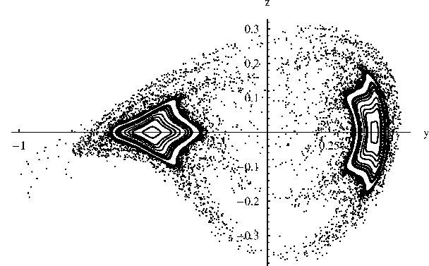 Figure 1
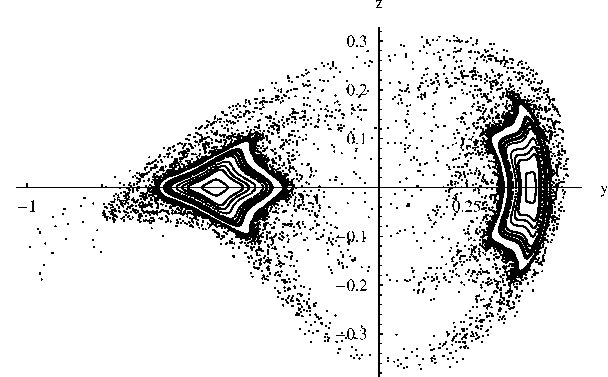 Figure 2
Peer Reviews
No public reviews on file for this paper yet. If you reviewed it on a platform where reviews are public (OpenReview, ICLR, NeurIPS, ICML), you can paste yours below so the community can read it here.
Videos
No videos yet. Explain this paper in a talk, walkthrough, or lecture? Add one.
Taxonomy
TopicsQuantum chaos and dynamical systems · Algebraic and Geometric Analysis · Numerical methods for differential equations
-Lohner algorithm
Daniel Wilczak111 Research supported by an annual national scholarship for young scientists from the Foundation for Polish Science , Piotr Zgliczyński222 Research supported in part by Polish State Ministry of Science and Information Technology grant N201 024 31/2163
Jagiellonian University, Institute of Computer Science,
Nawojki 11, 30–072 Kraków, Poland
e-mail: [email protected], [email protected]
Abstract
We present a Lohner type algorithm for the computation of rigorous bounds for solutions of ordinary differential equations and its derivatives with respect to initial conditions up to arbitrary order. As an application we prove the existence of multiple invariant tori around some elliptic periodic orbits for the pendulum equation with periodic forcing and for Michelson system.
1 Introduction
This paper is a sequel to [Z]. We present here a Lohner-type algorithm for computation of rigorous enclosures of partial derivatives with respect to initial conditions up to an arbitrary order of the flow induced by an autonomous ODE, hence the name -Lohner algorithm. Let be a positive integer, then by -algorithm we will mean the routine which gives rigorous estimates for partial derivatives with respect to initial conditions up to an order and -computations we mean an application of an -algorithm.
Our main motivation for the development of -algorithm was a desire to provide a tool, which will considerably extend the possibilities of computer assisted proofs in the dynamics of ODEs. Till now most of such proofs have used topological conditions (see for example [HZHT, MM, GZ, Z1]) and additionally conditions on the first derivatives with respect to initial conditions (see for example [RNS, T, Wi1, WZ, KZ]), hence it required - and -computations, respectively. The spectrum of problems treated includes the questions of the existence of periodic orbits and their local uniqueness, the existence of symbolic dynamics, the existence of hyperbolic invariants sets, the existence of homo- and heteroclinic orbits. To treat other phenomena, like bifurcations of periodic orbits, the route to chaos, invariant tori through KAM theory one needs the knowledge of partial derivatives with respect to initial conditions of higher order.
In principle, one can think that a good rigorous ODE solver should be enough. Namely, to compute the partial derivatives of the flow induced by
[TABLE]
it is enough to rigorously integrate a system of variational equations obtained by a formal differentiation of (1) with respect to the initial conditions. For example for we have the following system
[TABLE]
with the initial conditions
[TABLE]
It is well known that if by we denote the (local) flow induced by (1), then
[TABLE]
Analogous statements are true for higher order partial derivatives with respect to initial conditions.
It turns out that a straightforward application of a rigorous ODE solver to the system of variational Equations (2–4) is very inefficient. Namely, it totally ignores the structure of the system and leads to a very poor performance and unnecessary long computation times (see Section 4.1).
Our algorithm is a modification of the Lohner algorithm [Lo], which takes into account the structure of variational Equations (2–4). Basically it consists of the Taylor method, a heuristic routine for a priori bounds for solution of (2–4) during a time step and a Lohner-type control of the wrapping effect, which is done separately for and partial derivatives with respect initial conditions (the variables and in (3,4)). The Taylor method is realized using the automatic differentiation [Ra] and the algorithms for computation of compositions of multivariate Taylor series.
The proposed algorithm has been successfully applied in [HNW] to the Michelson system [Mi], where a computer assisted proof of the existence of a cocoon bifurcation was presented. Some parts of this proof required -computations.
In the present paper in Section 8 we show an application of our algorithm to pendulum equation with periodic forcing and the Michelson system. We used it to compute rigorous bounds for the coefficients of some normal forms up to order five, which enabled us to prove the existence of invariant tori around some elliptic periodic orbits in these systems using KAM theorem for twist maps on the plane. These proofs required and computations.
2 Basic definitions
To effectively deal with the formulas involving partial derivatives we will use extensively a notation of multiindices, multipointers and submultipointers throughout the paper.
As an motivation let us consider the formula for the partial derivatives of the composition of maps. Assume and are of class . We have
[TABLE]
To the operator we can in a unique way assign a multipointer, which is a nondecreasing sequence of integers , such that . A submultipointer is a multipointer, which is a part of a longer multipointer, for example . One observes, that submultipointers appear at several places in the above formula.
A multiindex is an element of . It is another way to represent various partial derivatives. The coefficient tells us how many times to differentiate a function with respect to the -th variable. Obviously, we have one-to-one correspondence between multipointers and multiindices.
2.1 Multiindices
By we will denote the set of nonnegative integers, i.e. .
Definition 1
An element will be called a multiindex.
For a sequence and a vector we set
2. 2.
3. 3.
By we will denote
[TABLE]
We will drop the index (the dimension) in the symbol when it is obvious from the context.
Put .
For we set
2. 2.
Let be sufficiently smooth. For we set
2. 2.
For a function by we will denote and similarly
[TABLE]
This convention means that always acts on -variables.
2.2 Multipointers
For a fixed and we define
[TABLE]
Definition 2
An element of will be called a multipointer.
Remark 3
A function
[TABLE]
is a bijection.
Let be a sufficiently smooth. For we set
2. 2.
For a function by we will denote . In the light of the above notations .
For and we define
[TABLE]
For and we define
[TABLE]
By we will denote a linear order (lexicographical order) in defined in the following way. For and
[TABLE]
Definition 4
For we set
[TABLE]
We will use extensively in the next section. Its will be used to label terms in . Observe that for
[TABLE]
One can construct all elements of using the following recursive procedure. From the definition of it follows that if then (notice that order is preserved). Similarly, if then
[TABLE]
and again order of elements is preserved. Hence, for and we have where
[TABLE]
and the sets and are disjoint.
Another way to generate all elements of can be described as follows
- •
decompose the set into nonempty and disjoints sets ,
- •
we sort each and permute ’s to obtain
- •
we define to be an ordered set consisting of all elements of for
Definition 5
For an arbitrary and such that we define a submultipointer by for , which can be expressed using as follows
[TABLE]
3 Equations for variations
Consider an ODE where is . Let be a local dynamical system induced by . It is well known, that and one can derive the equations for partial derivatives of by differentiating equation with respect to the initial condition . As a result we obtain a system of so-called equations for variations, whose size depends on the order of partial derivatives we intend to compute. An example of such system for is given by (2–4) with initial conditions given by (1).
The goal of this section is to write the equations for variations in a compact form using multipointers and multiindices, which allows us to take into account the symmetries of partial derivatives,
Lemma 6
Assume and let be a local dynamical system induced by . Then for such that holds
[TABLE]
for .
Proof: In the proof the functions are always evaluated at , and various partial derivatives of are always evaluated at , therefore the arguments will be always dropped to simplify formulae. We prove the lemma by induction on . If then for some and (9) becomes
[TABLE]
Assume (9) holds true for , . Let us fix . We have , where and . Since (9) is satisfied for , therefore we have
[TABLE]
For we set
[TABLE]
Now our goal is to prove that:
[TABLE]
Our strategy of proof is as follows. We will define , such that
[TABLE]
We set
[TABLE]
For we set
[TABLE]
It remains to show that for . Consider first . Recall that , hence
[TABLE]
Therefore
[TABLE]
Consider now . For an arbitrary contains only one element . Therefore we obtain
[TABLE]
Since , where , hence
[TABLE]
Consider now . We have
[TABLE]
Using decomposition as in (8) we obtain
[TABLE]
We have shown that for . This finishes the proof.
4 -Lohner algorithm
4.1 Why one needs an -algorithm?
There are several effective algorithms for the computation of rigorous bounds for solutions of ordinary differential equations, including Lohner method [Lo], Hermite–Obreschkoff algorithm [NJ] or Taylor models [BM]. For -computations the number of equations to solve is equal to hence, even for direct application of such an algorithms to equations for variations (14) leads to integration in high dimensional space and is usually inefficient. Let us recall after [Z, Sec. 6] the basic reason for this. In order to have a good control over the expansion rate of the set of initial conditions during a time step these algorithms, while being , are ’internally’(or higher for Taylor models), because they solve non-rigorously equations for () - the variational matrix of the flow. This effectively squares the dimension of phase space of the equation and impacts heavily the computation time. But as it was observed in [Z] the equations for partial derivatives of the flow can be seen as non-autonomous and nonhomogenous linear equations, therefore we do not need additional equations for variations for them. As a result the dimension of the effective phase space for our -algorithm is given by and not a square of this number.
Another important aspect of the proposed algorithm is the fact that the Lohner-type control of the wrapping effect is done separately for -variables and variables . This feature is not present in the blind application of algorithm to the system of variational equations and it turns out that this often practically switches off the control of the wrapping effect on -variables, as various choices used in this control become dominated by the -variables.
In [Z] a -algorithm has been proposed. Here we present an algorithm for computation of higher order partial derivatives.
4.2 An outline of the algorithm
Let us fix and consider the following system of differential equations
[TABLE]
for all , .
Our goal is to present an algorithm for computing a rigorous bound for the solution of (14) with a set of initial conditions
[TABLE]
In the sequel we will use the following notations:
- •
if a solution of system (14) is defined for and some , then for by we denote
- •
for by we will denote a set for which we have . This set is obtained using an rigorous numerical routine described below.
The -Lohner algorithm is a modification of -Lohner algorithm [Z]. One step of -Lohner is a shift along the trajectory of the system (14) with the following input and output data
Input data:
- •
- a current time,
- •
- a time step,
- •
, such that ,
- •
, such that for .
Output data:
- •
- a new current time,
- •
, such that ,
- •
, such that for .
We will often skip the arguments of when they are obvious from the context.
The values of and , are computed using one step -Lohner algorithm. After it is done, we perform the following operations to compute for
1.
Find a rough enclosure for .
2.
Compute , this will also involve some rearrangement computations to reduce the wrapping effect for [Mo, Lo].
5 Computation of a rough enclosure for
For a fixed multipointer Equation (14) can be written as follows
[TABLE]
where
[TABLE]
The procedure for computing the rough enclosure is based on the notion of a logarithmic norm, which we give below.
Definition 7
[HNW]** For a square matrix the logarithmic norm is defined as a limit
[TABLE]
where is a given matrix norm.
The formulas for the logarithmic norm of a real matrix in the most frequently used norms are (see [HNW])
for , 2. 2.
for m , is equal to the largest eigenvalue of 3. 3.
for ,
In order to find bounds for we use the following theorem [HNW, Thm. I.10.6]
Theorem 8
Let be a solution of a differential equation
[TABLE]
Let be a piecewise differentiable function with values in . Assume that
[TABLE]
where by , we denote a logarithmic norm of a square matrix .
Then for we have
[TABLE]
with .
We apply the above theorem to Equation (16) to obtain
Lemma 9
Let us fix . Assume that and , then for
[TABLE]
with .
Proof: Consider Equation (16) and a homogenous problem for (16)
[TABLE]
Using Theorem 8 we can estimate the difference between any solution of (21), , and a solution of (16), denoted by .
[TABLE]
After a substitution , which is a solution of the homogenous equation, we obtain our assertion.
Usually, we do not have any control over the time dependence of and , hence we will use the following
Lemma 10
Assume that and for then for we have
[TABLE]
or
[TABLE]
5.1 The procedure for the computation of the rough enclosure for .
The procedure for the computing of the rough enclosure is iterative, which means that given a rough enclosure for and rough enclosures for all we are able to compute the rough enclosure for for .
The procedures for computation of the rough enclosures of and for has been given in [Z]. Below we present an algorithm for computing for .
Input parameters:
- •
- a time step,
- •
- the current value of ,
- •
- a compact and convex such that
- •
, such that for .
Output:
- •
, such that
[TABLE]
Before we present an algorithm let us observe that for a fixed , defined in (17) could be seen as a multivariate function of , and for . More precisely, put , where stands for number of elements of a set. Recall that, we have defined by (6) a linear order in . Hence, there is a unique sequence of multipointers , such that for , and for .
Let us define
[TABLE]
by
[TABLE]
and
[TABLE]
Algorithm:
To compute for we proceed as follows
1.
Find .
2.
Compute , i.e.
[TABLE]
For example, if , then should be such that
[TABLE]
3.
Define , for , where denotes -th coordinate of .
One can refine the obtained enclosure by
[TABLE]
Indeed, for , and we have
[TABLE]
for some . In the above we have used the fact that
[TABLE]
Since and for we get
[TABLE]
6 Computation of
6.1 Composition formulas
For any -times continuously differentiable functions and we have
[TABLE]
We can apply the above formula to and to obtain
[TABLE]
for all . Using notations and we can rewrite the above equation as
[TABLE]
where is defined by (5).
6.2 The procedure for computation of
We introduce new parameters - the order of the Taylor method used in computations of for . It makes sense to take .
Input parameters:
- •
- a time step,
- •
- the current value of ,
- •
- a current value of , for
- •
compact and convex, such that - a rough enclosure for ,
- •
, compact and convex, such that , for .
Output: , such that
[TABLE]
for and .
Algorithm: We compute as follows
1.
Computation of using Taylor method for Equation (14), i.e. for we compute
[TABLE]
where for and for . Observe that
[TABLE]
Indeed, using Taylor series expansion we obtain that for and holds
[TABLE]
for some . Observe, that
[TABLE]
Using and for we obtain our assertion.
2.
The composition. Put
[TABLE]
Using (28) for we have
[TABLE]
where
[TABLE]
In our implementation of the algorithm we use the symbolic differentiation to obtain formulae for . Next, using the automatic differentiation we compute which appear in (1.).
6.3 Rearrangement for - the evaluation of Equation
(32)
It is well know that a direct evaluation of Equation (32) leads to wrapping effect [Mo, Lo]. To avoid it following the work of Lohner [Lo] we will use the same scheme as it was proposed in [Z].
Namely, observe that Equation (32) has exactly the same structure as the propagation equations for -method (see [Z, Section 3]). Moreover, all vectors , for ’propagate’ by the same as did the variational part in [Z], hence it makes sense the same approach.
To be more precise, each set , for is represented in the following form
[TABLE]
where is interval matrix, is point matrix, is a point vector and are interval vectors. Observe that and are independent of .
In the sequel we will drop index . Equation (32) leads to
[TABLE]
Let denotes a center of an interval object, i.e. is interval vector or interval matrix and .
Let be an interval matrix which contains an orthogonal matrix. Usually, is computed by the orthonormalisation of the columns of .
Let
[TABLE]
Then we rearrange formula (34) as follows
[TABLE]
Summarizing, we can use the following data structure to represent and , for
type CnSet = record
: IntervalVector;
: IntervalMatrix;
end;
The set is represented as , the partial derivatives are represented as . The matrices are common for all partial derivatives.
Notice, that if we start the computation with an initial condition (15) then there is no Lipschitz part at the beginning for the partial derivatives. Hence, the initial values for and are set to the identity matrix and the initial values for are set to zero.
If the interval vectors become ’thick’ (i.e. theirs diameters are larger than some threshold value) we can set a new Lipschitz part in our representation (it must be done simultaneously for all ) and reset in the following way
[TABLE]
A similar change of the Lipshitz part may be done when vectors become thick in comparison to .
7 Derivatives of Poincaré map
Consider a differential equation
[TABLE]
Let be a (local) dynamical system induced by (36). Let be -map. Put .
Definition 11
We will say that is a local section for the vector field at if
[TABLE]
Assume and are such that is a local section at . Consider an implicit equation
[TABLE]
It follows easily from (37) and from the implicit function theorem that there exists a uniquely defined in a neighborhood of , such that . The function is as smooth as the flow . We will refer to as to the Poincare return time to section .
We define a Poincaré map by
[TABLE]
Usually the Poincaré map is defined as a map , where are local sections in . The approach taken here, i.e. treating the Poincaré map as map allows us to not to worry about the coordinates on local section.
In this section we are interested in the partial derivatives of defined by (39).
From (39) we can compute and we obtain
[TABLE]
We need . We differentiate (38) to obtain
[TABLE]
Hence
[TABLE]
7.1 Higher order derivatives of the Poincaré map
To make formulas transparent we will drop arguments of functions in this section, but reader should be aware that for and its partial derivatives the argument is , for and the argument is always the pair .
From (40) we obtain
[TABLE]
It is easy to see that partial derivatives of high order give rise to quite complex expressions and it is not entirely obvious how to organize it in some coherent and programmable way. For this purpose we use the following
Lemma 12
For a multipointer we have
[TABLE]
Proof: By induction on . For formula (43) is equivalent to (40), because the two last sums are taken over empty set. Assume (43) holds true for some and fix . Our goal is to show that
[TABLE]
where
[TABLE]
Write , where and . From the induction assumption we have
[TABLE]
where
[TABLE]
Obviously . We will show that and .
Denote by , a part of sum with fixed . Similarly, let us denote by a part of sum , , for .
Using decomposition of as in (8) we obtain that . Similarly, using (8) we observe that for . Finally, since and we find that . This shows that .
It remains to show that . We will classify possible terms by the fact, where appears in , and how this enters in as or . There are four cases
2. 2.
3. 3.
, 4. 4.
,
Let us fix . Let . The term for case 1 is , for case 2 is , case 3 is and case 4 is . Hence, .
For and fixed we have: case 1 is given by , case 2 by , case 3 by and case 4 by Hence, for we have .
Finally, for we observe, that . Indeed, in this case . Hence, either for we have term and we have .
We have showed that and the proof is finished.
Hence, if we know all the partial derivatives of up order we can compute the partial derivatives of the Poincaré map up the same order. In next subsection we show how to compute partial derivatives of for affine sections.
7.2 Partial derivatives of for affine sections
Assume is an affine map given by
[TABLE]
This is a quite restrictive assumption about sections, but it leads to relatively simple formulas for and it is sufficient for the applications we have in mind.
Lemma 13
For a multipointer holds
[TABLE]
Proof: The proof is a direct consequence of Lemma 12 and (38). Since is affine, by differentiating of we get . Using formula (43) for we obtain our assertion.
Fix and assume we have a rigorous bound for (see [Z, Section 6] for more details on this). Lemmas 13 and 12 show that given rigorous bounds for the partial derivatives and up to some order we can compute recursively rigorous bounds for the partial derivatives of and up to the same order. Notice, that are given by Taylor coefficients of the solution of (14) with initial conditions for part and for equations for variations. Hence, these coefficients can be easily computed using the automatic differentiation algorithm.
8 Applications.
One of the typical invariant sets in hamiltonian mechanics are invariant tori. However, the existence of invariant torus in a given system is often difficult to prove despite the fact that the theory is quite well developed. Probably the best work in this direction was done by Celletti and Chercia [CC1, CC2], where the an effective application (computer assisted proof) of KAM theory to the restricted three body problem modelling system consisting of Sun, Jupiter and asteroid 12 Victoria was given. Our aim here is more modest as we focus on the invariant tori emanating from the elliptic fixed point satisfying suitable twist condition.
In this section we show that the rigorous computations of partial derivatives of a dynamical system up to order or can be used to prove that in a particular system an invariant torus exists around some elliptic periodic orbits. In this section this will be done for the forced pendulum equation and the Michelson system.
8.1 Area preserving maps on the plane, normal forms and KAM theorem
Definition 14
Let be a smooth area preserving map, such that . Let and be eigenvalues of . Following [SM] we will call the point
- •
hyperbolic* if and ,*
- •
elliptic* if and ,*
- •
parabolic* if .*
The following KAM theorem will be the main tool to prove the existence of invariant tori in this paper.
Theorem 15
[SM, §32]** Consider an analytic area preserving map , where
[TABLE]
and denotes convergent power series in with terms of order greater than , only.
If at least one of is not zero then the origin is a stable fixed point for map . Moreover, in any neighborhood of point [math] there exists an invariant curve for map around the origin contained in .
The next theorem and its proof tells how to bring a planar area preserving map in the neighborhood of an elliptic fixed point into the form (44).
Theorem 16
[SM, §23]** Consider an analytic area preserving map such that . Let be complex eigenvalues of , such that . If for , then there is an analytic area preserving substitution such that in the new coordinates mapping has form (44).
The proof of the above theorem is constructive, i.e. given the power series for at an elliptic fixed point one can construct explicitly an area preserving substitution and compute the coefficients in (44). An explicit formula for the coefficient in the above normal form is given in Appendix A.
8.2 The existence of invariant tori in forced pendulum.
Consider an equation
[TABLE]
Observe that (45) is hamiltonian.
Let us denote by the Poincaré map for Equation (45) with a parameter , i.e. , where is a local flow induced by (45). Observe that (45) is nonautonomous, but it is equivalent to first order system of autonomous ODE given by
[TABLE]
In the sequel all rigorous computations for (45) will be in fact performed for the system (46).
Observe that to any invariant closed curve for corresponds and invariant 2-torus for (45).
Consider a set of parameter values
[TABLE]
The following lemma was proved with computer assistance
Lemma 17
For all parameter values there exists an elliptic fixed point for . Moreover, there exists an area-preserving substitution such that in the new coordinates the map has the form (44) with and .
Before we give the proof, let us briefly comment about the choice of the parameter set . For parameter values slightly lower than we observe the parabolic case, i.e. there exists a parameter value for which eigenvalues of the derivative of are equal to . In two gaps in below and we have resonances of low order. Namely, we have parameter values with an elliptic fixed with eigenvalues to and , respectively. Clearly, in a computer assisted proof we need to exclude a small interval around those parameters. For it seems that the interval can be extended much further to the right without any difficulty.
Proof of Lemma 17: A computer assisted proof consists of the following steps. We cover the set by nonequal subintervals . Diameters of ’s were relatively large for values far away from the parabolic cases and very small close to them. For a fixed subinterval we proceed as follows
Let denote an approximate center of the interval . We find an approximate fixed point for using the standard nonrigorous Newton method. Let us denote such a point by . 2. 2.
We define a box centered at , i.e we set , where depends on subinterval - the values we used are from the interval , depending on whether close to parameter values corresponding to parabolic cases. 3. 3.
Using the -Lohner algorithm we compute the Interval Newton operator [Mo, N, A] and verify that . This proves that for all there exists a unique fixed point for . 4. 4.
Using the -Lohner algorithm we compute a rigorous bound for and , . Hence, we obtain a rigorous bound for the coefficients in
[TABLE] 5. 5.
We show that an arbitrary matrix has a pair of complex eigenvalues which satisfy for . From Theorem 16 it follows there exists an area-preserving substitution such that in the new coordinates the map for has the form (44) with . 6. 6.
We compute a rigorous bound for and which appear in the formula (44) and verify that for holds .
The rigorous bounds for the values of on are
[TABLE]
A computer assisted proof of the above took approximately minutes on the Pentium IV 3GHz processor.
As a straightforward consequence of Lemma 17 and Theorem 15 we obtain
Theorem 18
For all parameter values there exists an elliptic fixed point for . Moreover, any neighborhood of point contains an invariant curve for around .
8.3 Higher order normal forms.
In the previous section it was shown that computations are sufficient to prove that for (45) a family of invariant tori exists. However, it may happen that the coefficient in the normal form vanishes. In this situation we may try to compute higher order normal form. As an example we consider a pendulum with a different forcing term,
[TABLE]
Theorem 19
Let be the Poincaré map for (47). For all parameter values there exists an elliptic fixed point for . Moreover, any neighbourhood of point contains an invariant curve for around .
Proof: The main concept of the proof is the same as in Lemma 17. Using the nonrigorous Newton method we find an approximate fixed point
[TABLE]
We set . Using the -Lohner algorithm we compute the Interval Newton Operator of on and we obtain that for all , , where
[TABLE]
Since we conclude that for all there exists a unique fixed point for the Poincaré map.
Using -Lohner algorithm we compute a rigorous bound for and , . Hence, we obtain a rigorous bound for the coefficients in
[TABLE]
We show that an arbitrary matrix has a pair of complex eigenvalues which satisfy for . From Theorem 16 it follows there exists an area-preserving substitution such that in the new coordinates the map for has the form (44) with .
Next, we compute a rigorous bound for and which appear in the formula (44) and we get
[TABLE]
Since for , the assertion follows from Theorem 15.
The main observation which makes this example interesting is that there exists for which and we cannot conclude the existence of invariant tori for all from computations. To be more precise, we computed the coefficient for the parameter values and and we get
[TABLE]
Since exists for all and depends continuously on we conclude, that for some .
8.4 Application to the Michelson system
The existence of an invariant curve for a planar map can be proven without assumption that is measure preserving. The key assumption in the proof given in [SM] is that any curve around an elliptic point intersect its image under , i.e. . Such a situation is also observed in reversible planar map around an symmetric elliptic fixed points.
Definition 20
An invertible transformation is called a reversing symmetry of a local dynamical system , or if the following conditions are satisfied
if then . 2. 2.
**
Remark 21
In the discrete time case, the above two conditions are equivalent to identity
[TABLE]
where is a generator of .
Definition 22
Let be a local (discrete or continuous) dynamical system. For put
[TABLE]
The set will be called a trajectory of a point .
Definition 23
Assume is an reversing symmetry for . An orbit is called -symmetric orbit if .
Remark 24
[La]** In continuous case the orbit is -symmetric if it contains a point from the set .
Remark 25
[Wi2, Lem.3.3]** It is easy to see that if is a Poincaré section for a -reversible flow such that then the Poincaré map is -reversible.
As we observed at the beginning of this section, an -reversible planar map may admit an invariant curve around an -symmetric elliptic fixed point. In reversible case a planar map admits the same normal form around symmetric, elliptic fixed point as in the area-preserving case and the substitution which tends the map to the normal form is exactly the same as we described in Appendix A – for details see [Se, BHS].
Consider an ODE
[TABLE]
On one hand, the system (48) is an equation for the steady state solution of one-dimensional Kuramoto-Sivashinsky PDE and it is known in the literature as the Michelson system[Mi]. On the other hand, this system appears as a part of the limit family of the unfolding of the nilpotent singularity of codimension three (see [DIK1]).
The system (48) is reversible with respect to the symmetry
[TABLE]
and since the divergence vanishes it is also volume preserving.
A dynamical system induced by (48) exhibits several types of dynamics for different values of parameter. For sufficiently large there is a simple invariant set consisting of two equilibria and heteroclinic orbit between them [MC]. Lau [Lau] numerically observed that when the parameter decreases a cascade of cocoon bifurcations occurs and at the limit value a periodic orbit is born through a saddle-node bifurcation. This hypothesis has been proved in [KWZ]. The computer assisted proof of this fact given in [KWZ] uses the algorithm presented in this paper in order to compute partial derivatives up to second order for a certain Poincaré map.
For the parameter value equal to one and slightly smaller than one it was proven in [DIK2, Wi1, Wi2, Wi3] that the system has rich and complicated dynamics including symbolic dynamics, heteroclinic solutions, Shilnikov homoclinic solutions.
However, as the bifurcations diagram presented by Michelson suggests [Mi, Fig.1] for all parameter values there are at least two elliptic periodic orbits with large invariant islands around them. In this section we present a proof that such islands exist for some range of parameter values. The main idea of the proof is almost the same as in the previous section. There are two main differences. First, the Poincaré map will not be a time shift. Therefore computations of the partial derivatives of the Poincaré map require Lemma 12 and Lemma 13. Second difference is: we use the shooting method instead of the interval Newton method for the proof of the existence of symmetric periodic orbit.
The aim of this section is to prove the following
Theorem 26
For all parameter values from the set
[TABLE]
there exists a symmetric elliptic periodic orbit for the Michelson system (48). Moreover, each neighbourhood of such an orbit contains a tori invariant under the flow generated by the Michelson system.
Let us define the Poincaré section . Let be the Poincaré map for the system with the parameter value . Notice, that is in fact a half Poincaré map, which means that the trajectory of crosses in opposite directions when passing through and , and therefore periodic orbits for the Michelson system corresponds to periodic points for .
Since the section is invariant under symmetry , from Remark 25 the Poincaré map is also reversible with respect to an involution . We will use the same letter to denote the reversing symmetry of the Poincaré map and the Michelson system.
Let us comment about the choice of the set . In the gap between intervals and there is a parameter value for which the eigenvalues of the Poincaré map are . Apparently at this parameter value we have a bifurcation and four periodic islands are born as it is shown in Fig.1 - see also a movie mpp.mov available at [Wi4] which presents an animation of the phase portrait of for the parameter values from the range .
Proof of Theorem 26. The main concept of the proof is quite similar to the one presented in Lemma 17. We divide the set of parameter values onto nonequal parts (smaller when close to the bifurcation parameter and close to and ). For a fixed subinterval from the grid we proceed as follows
Let denote a center of the interval . We find an approximate fixed point of using the standard nonrigorous Newton method. Let us denote this point by . 2. 2.
Since the map is reversible one can prove the existence of the fixed point for using the shooting method as follows.
Let . Since satisfies whenever the left side is defined, one can see that if and then . Let us remark, that we always get an approximate fixed points resulting from the nonrigorous Newton method very close to . We define two points , where is a small number depending on and we show that , where is a projection onto coordinate. Hence, if the is defined on the set then for all parameter values there is a point which satisfies and therefore . This shows that for all there exists a fixed point for inside provided is defined on , which will be discussed below. 3. 3.
Using -Lohner algorithm we compute rigorous bounds for and for . This implies also that . 4. 4.
We show that an arbitrary matrix has a pair of complex eigenvalues which satisfy for . From Theorem 16 it follows there exists an area-preserving substitution such that in the new coordinates the map for has the form (44) with . 5. 5.
We compute a rigorous bound for and which appear in the formula (44) and verify that for holds .
The rigorous bounds for the values of on are
[TABLE]
The computer assisted proof of the above took approximately hours and minutes on the Pentium IV 3GHz processor.
9 Implementation notes.
All the algorithms presented in this paper have been implemented in C++ by authors and are part of the CAPD library [CAPD]. In particular, the package implements the computation of partial derivatives of a flow with respect to initial condition, partial derivatives of Poincaré maps for linear sections and computations of normal forms for planar maps up to order .
The implementation combines the automatic and symbolic differentiation in order to generate a coefficients in Taylor series for the solutions of the system (14).
Our tests shows that without difficulty we can compute partial derivatives up to order for an equation in -dimensional phase space (which gives equations to solve) on a computer with 512MB memory. However, our current implementation is optimized for lower dimensional problems. All the trees which represent formulas (14) are stored in the memory of a computer. This speeds up computations because we do not need to recompute all the multiindices, multipointers and submultipointers in each step of the algorithm. Unfortunately, such an implementation is memory-consuming. Therefore, higher dimensional problems require a computer with huge memory even for or computations.
Appendix A Explicit formulas for third order normal forms for a planar
map
The goal of this section is to give some details about the proof of Theorem 16. We want to present some formulas to give the reader the feeling about the necessary computations.
Throughout this section we assume that the assumptions of Theorem 16 are satisfied. In the neighbourhood of [math] is given by a real, convergent power series
[TABLE]
Denote also by a complex extension of . Let be complex eigenvalues of and corresponding eigenvectors (here bar denotes the complex conjugation). Then, using a linear substitution of the form , we can change the coordinate system such that in the new coordinates the mapping has the form
[TABLE]
The last condition is a consequence of the invariance of under the complex map . We will refer to it as the reality condition. Namely, the set in the new coordinates is given by and the condition expressed in coordinates is equivalent to (A).
Assume now, that for . Then an analytic area-preserving substitution satisfying reality condition (A)
[TABLE]
where
[TABLE]
brings to the normal form
[TABLE]
with
[TABLE]
Finally, let be such that and we compute coefficient by
[TABLE]
From the proof given in [SM] it follows that and the mapping in coordinates has the form
[TABLE]
where is a convergent power series with the terms of degree at least .
Again, the coefficients of satisfy reality condition (A). In order to express this normal form in terms of real variables we make a linear substitution
[TABLE]
and we obtain the normal form for
[TABLE]
which agrees with (44).
The formulas for higher order terms (and for , which are not given here) has been computed in Mathematica.
The reference list from the paper itself. Each links out to its DOI / PubMed record.
- 1[A] G. Alefeld, Inclusion methods for systems of nonlinear equations - the interval Newton method and modifications , in Topics in Validated Computations, J. Herzberger (Editor), Elsevier Science B.V., 1994, pages 7–26
- 2[BHS] H.W. Broer, G.B. Huitema and M.B. Sevryuk, Quasi-periodicity in families of dynamical systems: order amidst chaos , Lecture Notes in Mathematics, Vol. 1645, Springer Verlag, (1996).
- 3[BM] M. Berz, K. Makino, New Methods for High-Dimensional Verified Quadrature , Reliable Computing, 5, 13-22 (1999)
- 4[CAPD] CAPD – Computer Assisted Proofs in Dynamics group, a C++ package for rigorous numerics, http://capd.wsb-nlu.edu.pl.
- 5[CC 1] A. Celletti, L. Cherchia, KAM Stability for three-body problem of the Solar System , Z. angw. Math. Phys. 57 (2006) 33-41
- 6[CC 2] A. Celletti, L. Cherchia, KAM Stability and Celestial Mechanics , Memoirs of the AMS, Vol 187, Num 878 (2007)
- 7[DIK 1] F. Dumortier, S. Ibáñez, and H. Kokubu, New aspects in the unfolding of the nilpotent singularity of codimension three, Dynam. Syst. 16 (2001), 63–95.
- 8[DIK 2] F. Dumortier, S. Ibáñez, and H. Kokubu, Cocoon bifurcation in three dimensional reversible vector fields , Nonlinearity 19 (2006), 305–328.