An Inverse $f(R)$ Gravitation for Cosmic Speed up, and Dark Energy Equivalent
Sohrab Rahvar, Yousef Sobouti

TL;DR
This paper introduces an inverse $f(R)$ gravity approach to explain cosmic acceleration by reconstructing the gravity function from observationally motivated scale factors, comparing it with standard dark energy models.
Contribution
It proposes a novel inverse $f(R)$ method to derive gravity functions from empirical scale factors, offering an alternative to dark energy explanations for cosmic acceleration.
Findings
Reconstructed $f(R)$ functions consistent with observed cosmic acceleration.
Identified dark energy parameters needed to match modified gravity models.
Compared modified gravity and dark energy scenarios to explain cosmic speed up.
Abstract
To explain the cosmic speed up, brought to light by the recent SNIa and CMB observations, we propose the following: a) In a spacetime endowed with a FRW metric, we choose an empirical scale factor that best explains the observations. b) We assume a modified gravity, generated by an unspecified field lagrangian, . c) We use the adopted empirical scale factor to work back retroactively to obtain , hence the term `Inverse '. d) Next we consider the classic GR and a conventional FRW universe that, in addition to its known baryonic content, possesses a hypothetical `Dark Energy' component. We compare the two scenarios, and find the density, the pressure, and the equation of the state of the Dark Energy required to make up for the differences between the conventional and the modified GR models.
Click any figure to enlarge with its caption.
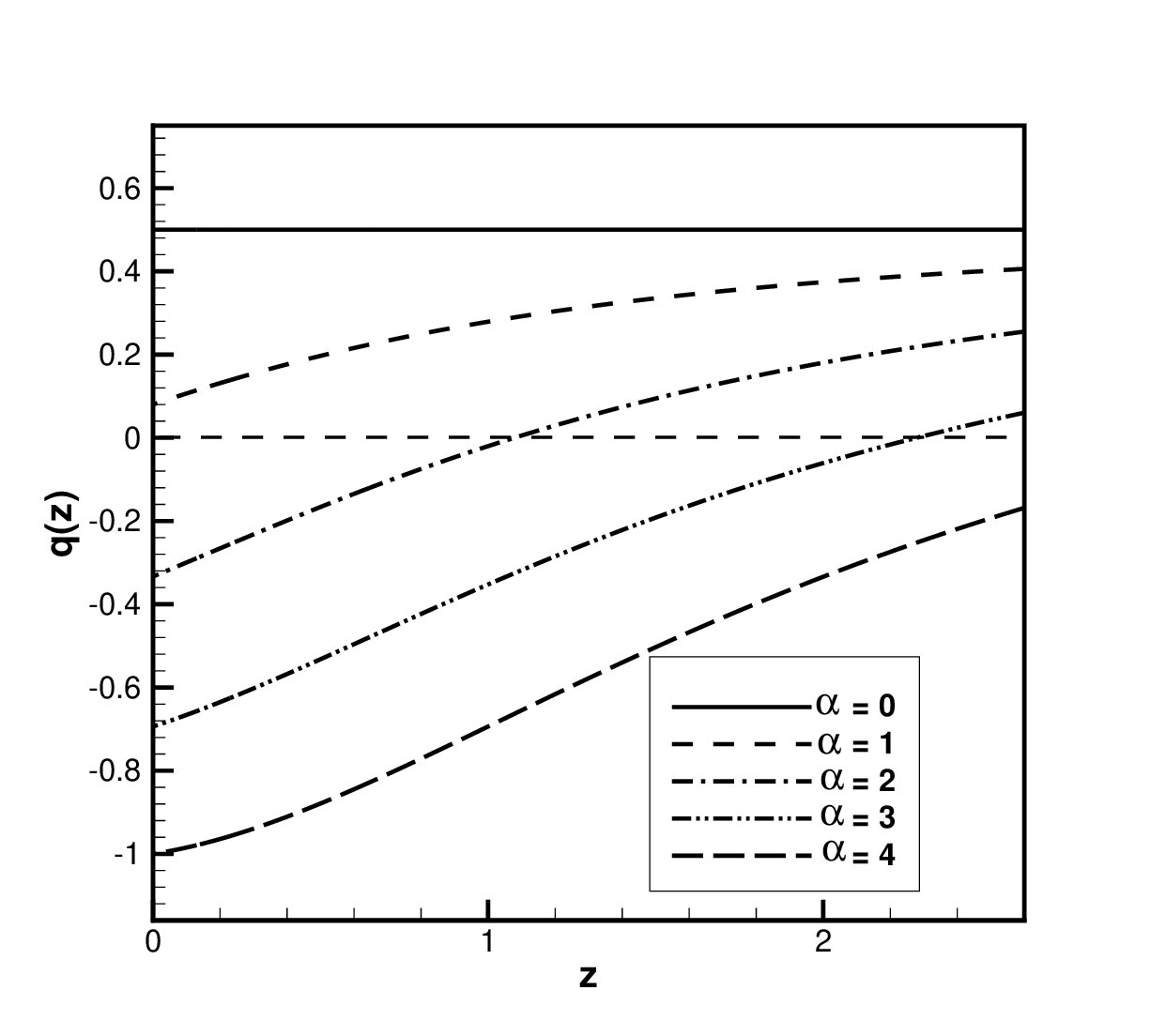 Figure 1
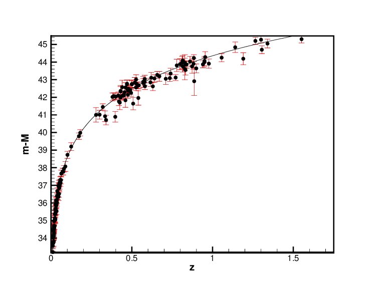 Figure 2
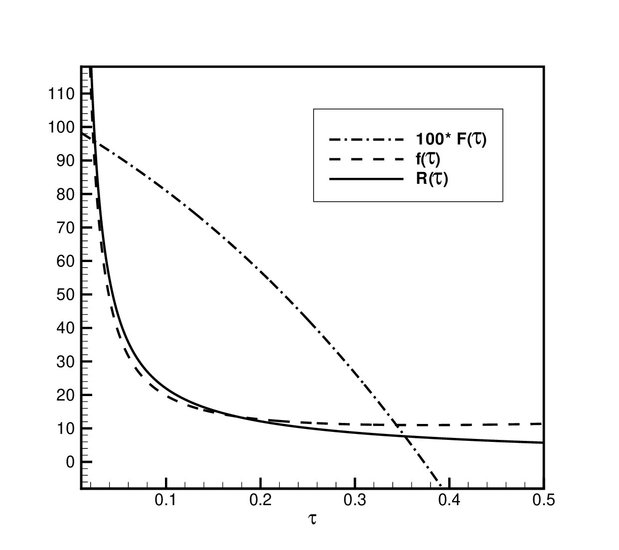 Figure 3
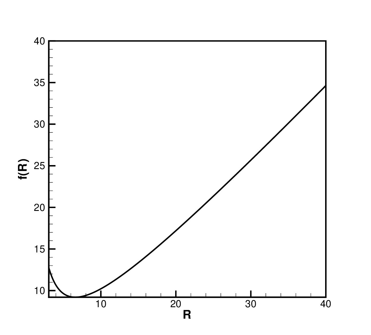 Figure 4
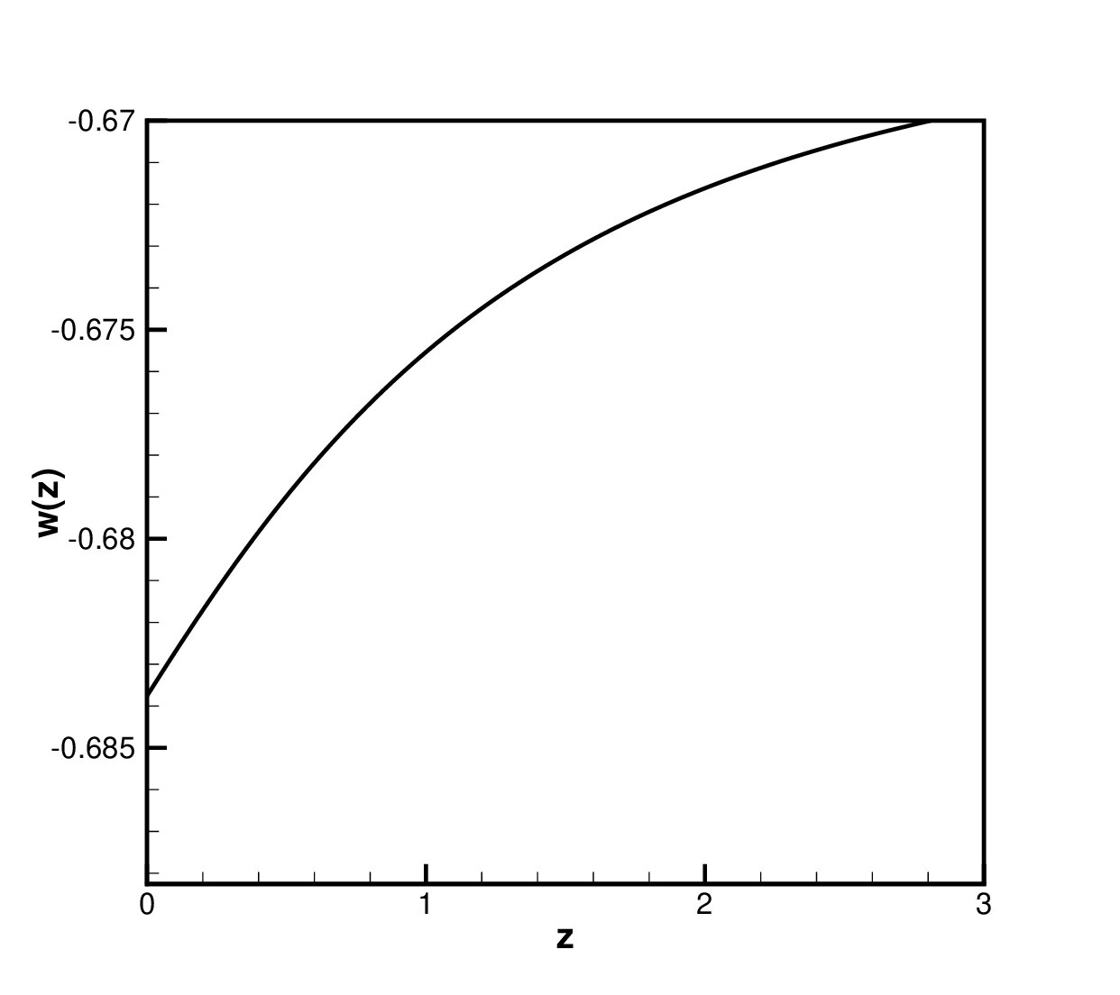 Figure 5
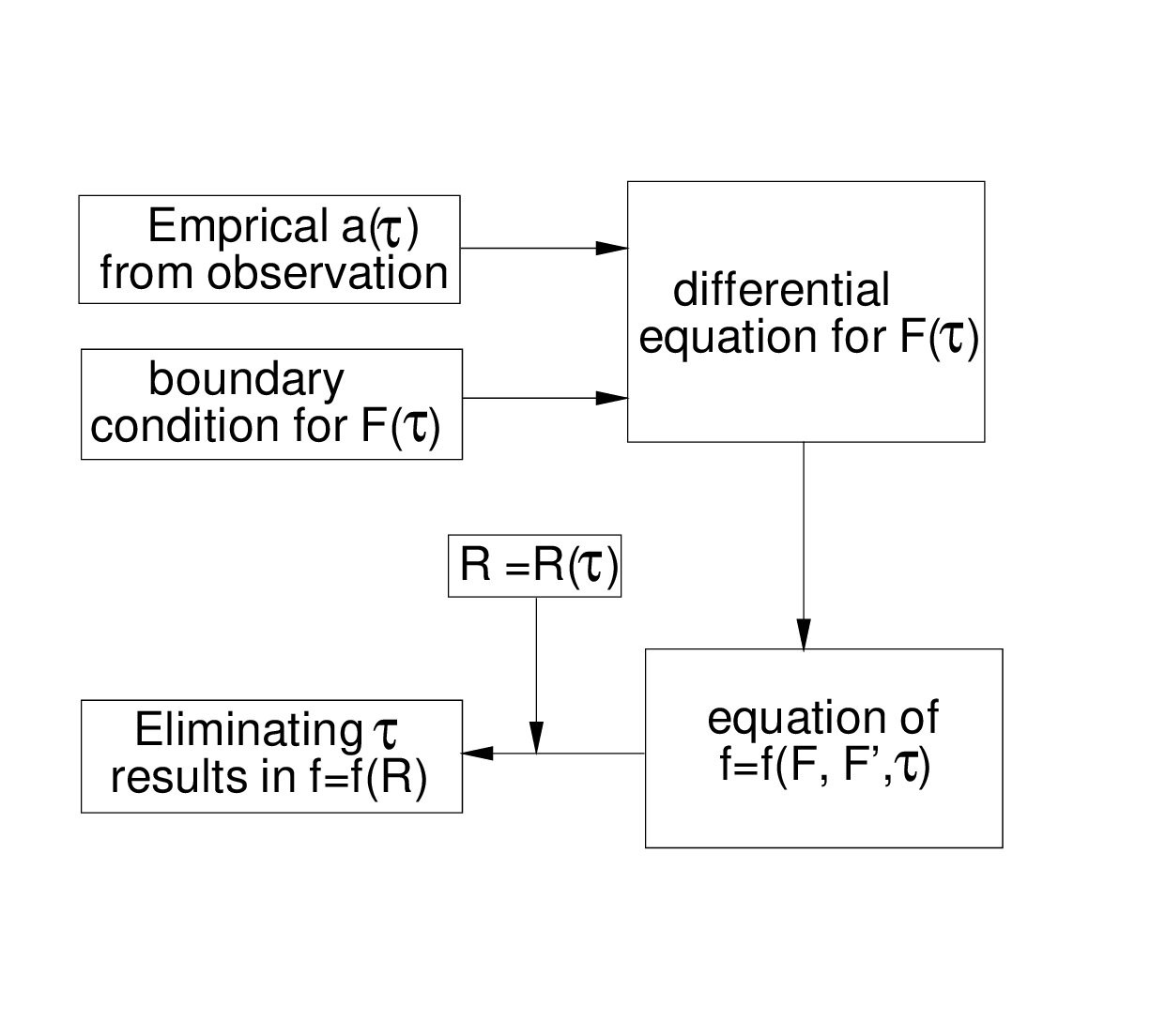 Figure 6
Peer Reviews
No public reviews on file for this paper yet. If you reviewed it on a platform where reviews are public (OpenReview, ICLR, NeurIPS, ICML), you can paste yours below so the community can read it here.
Videos
No videos yet. Explain this paper in a talk, walkthrough, or lecture? Add one.
\catchline
An Inverse Gravitation for Cosmic Speed up, and
Dark Energy Equivalent
Sohrab Rahvar
Department of Physics, Sharif University of Technology, P.O.Box 11365-9161, Tehran, [email protected]
Yousef Sobouti
Institute for Advanced Studies in Basic Sciences,
P.O.Box 45195-1159, Zanjan, Iran
Abstract
To explain the cosmic speed up, brought to light by the recent SNIa and CMB observations, we propose the following: a) In a spacetime endowed with a FRW metric, we choose an empirical scale factor that best explains the observations. b) We assume a modified gravity, generated by an unspecified field lagrangian, . c) We use the adopted empirical scale factor to work back retroactively to obtain , hence the term ‘Inverse ’. d) Next we consider the classic GR and a conventional FRW universe that, in addition to its known baryonic content, possesses a hypothetical ‘Dark Energy’ component. We compare the two scenarios, and find the density, the pressure, and the equation of the state of the Dark Energy required to make up for the differences between the conventional and the modified GR models.
keywords:
Cosmology; Dark Energy; Modified Gravity.
\pub
Received (Day Month Year)Revised (Day Month Year)
\ccode
95.36.+x, 98.80.Jk, 98.80.Es
As cosmological standard candles, supernovae type Ia (SNIa) appear dimmer than what one expects from a Cold Dark Matter (CDM) model of the universe [1, 2, 3]. This observation and other evidences from the Cosmic Microwave Background (CMB) measurements indicate that the universe is in an acceleration phase of its expansion [4, 5, 6]. A conventional CDM scenario does not explain this speed up. Some authors have stipulated a dark energy component to make up for whatever dynamical effects that the known energy momentum content of the model leaves unaccounted for [7, 8, 9, 10, 11, 12, 13, 14, 15, 16, 17, 18, 19, 20, 21]. Others have entertained alternatives to Einstein’s gravitation [22, 23, 24, 25, 26, 27, 28, 29, 30]. Yet a third school have resorted to inhomogeneous FRW universes to explain the dilemma [31]. Since all these approaches attempt to answer the same question, all should be equivalent, and there should be a way to translate one language to the other.
Here, we are concerned with the ’dark energy’ and ’alternative gravitation’ scenarios. We suggest to begin with a Freidman- Robertson- Walker (FRW) universe, to choose its scale factor, , in a way that best explains the available observations, and to work out the dynamics of the spacetime. Next, to write down the field equations for a modified gravitation, and knowing , to solve for . Finally, to attribute whatever deviations from the conventional FRW results there is, to a dark energy field, and to obtain its density, pressure, equation of state, etc.
**The choice of the scale factor
**In a FRW metric, , single term scale factors of the form lead to constant deceleration parameters, , and do not serve the purpose. We propose the following two-term ansatz
[TABLE]
where is the age of the universe, and and are the free parameters of the model, to be adjusted to ensure compatibility of the emerging results with observations. The factor is introduced to have . By letting either or tend to zero, one recovers the standard CDM universe. Hereafter, for economy in writing, we will use the time parameter instead of the conventional time . From Eq. (1) one finds
[TABLE]
For , can become negative and remain nonsingular throughout. Transition from a decelerated phase of expansion to an accelerated one takes place at or . For , is always positive and nonsingular. For , q can become negative but also singular. The last two possibilities are discarded. For all values of and ,
[TABLE]
In Fig.(1) we have plotted versus the redshift, , for several values of and .
As to and , both remain positive for all times. Both tend to as and decease monotonically to [math] as . They exhibit a normal behavior in the neighborhood of .
Equation (3), written for the present epoch, reveals a constraint on and , that should be observed in the final design of the model. Thus,
[TABLE]
**Empirical values of &
**The distance modulus (corrected for the reddening) and the (dimensionless) luminosity distance, , of supernovae are related as
[TABLE]
In Fig. (2), the observed distance modulus of 157 SNIa of Gold’s sample are plotted versus the redshifts. The solid curve is the plot of equation (7), in which, in compliance with the constraint of Eq. (6), we have chosen
[TABLE]
The fit to the data points is adequate for our purpose, though the parameters can be refined to optimize the fit. These numbers give and . On adopting , one obtains an age of for the universe.
**An inverse way out
**We begin with a modified field equation generated by an, as yet, unspecified field lagrangian, ,
[TABLE]
where , and . For a universe of FRW type, filled with a perfect fluid of density and pressure , Eq. (An Inverse Gravitation for Cosmic Speed up, and Dark Energy Equivalent) and the equation of continuity reduce to
[TABLE]
We further neglect the pressure and integrate Eq. (12) to obtain . Next we substitute for in Eq. (11), assume , change the time variable to , and find
[TABLE]
where the now stands for , and we have, arbitrarily, put the dimensionless constant , that appear in the course of mathematical manipulations equal to . We will shortly discuss the numerical solution of Eq. (An Inverse Gravitation for Cosmic Speed up, and Dark Energy Equivalent). Some general remarks on its asymptotic behavior, however, are instructive. As we find
[TABLE]
where and are calculable polynomials in , and begin with term 1; and are constants of integration to be obtained from boundary conditions. The exponents, and are approximate solutions of the indicial equation, . As , diverges to or converge to [math] on account of one or the other term. This feature makes the solutions sensitive to a CDM type boundary conditions of the form, and . Presently we have no basis, observational or otherwise, to make an intelligent guess as to what the appropriate boundary conditions are. For the sake of argument, however, we have adopt , and kept only the proper solution of Eq. (12). With known, Eq.(10) becomes an algebraic equation to calculate . The numerically calculated solutions of , and are plotted in Fig. (3). Elimination of in favor provides and
It is instructive to examine the asymptotic behavior of and analytically. In the limit of small and large ’s, corresponding to large and small ’s, one finds
[TABLE]
Note that is a dimensionless scalar as it should be. With known, it is a matter of simple integration to obtain . Thus,
[TABLE]
At early epochs (large ’s), the spacetime approaches the conventional FRW universe with the classical GR while for the later times we have a positive acceleration universe. Another point about this action is that for in the solar system scales, and . In this case we will have standard GR equation and evades from the solar system test. Recently this type of models have been studied by introducing action in the form of , where for in the solar system, and for larger ’s, in cosmological scales and inside the large scale structures the action reduces to [32, 33].
In the remaining range of , integration is done numerically and the results are plotted in Fig. (4).
**Dark Energy equivalent
**Instead of the modified gravitation considered above, let us assume a classic FRW universe. That is, let and . Let this universe, however, have a ’Dark Energy’ component, in addition to its conventional baryonic content. The counterparts of Eqs. (10), and (11) will be
[TABLE]
Subtracting Eq. (10) from (19), and Eq. (11) from (20) gives
[TABLE]
The equation of state for the dark energy is obtained by eliminating , implicit in and , between Eqs. (21) and (23). This is done numerically and as a function of the redshift is plotted in Fig. (5).
**Concluding remarks
**The algorithm of Fig. 6 summarizes the path we have followed in this letter.
We have resorted to the SNIa observations to design an empirical FRW metric that allows the model universe to transit from a phase of decelerated expansion at early epochs to an accelerated one at later times. The spacetime is almost a CDM model and the gravity is almost the classic GR at very early times, but evolves away in course of time. Next we have maintained that the so-designed spacetime is deducible from a modified non- Hilbert- Einstein field lagrangian, . Knowing the metric, we have solved the modified field equations retroactively for the sought-after . Finally, we have compared our results with those of a conventional FRW model and have attributed the differences between the two to a dark energy component. Eventually, we have extracted the density, the pressure, and the equation of state of this stipulated energy.
We note that our choice of the scale factor and the adjustment of its free parameters, to comply with the available cosmological observations, is, by no means, unique. The goal is simply to demonstrate that the use of the observations at the outset, to deduce the rudiments of what seems reasonable, facilitates the access to possible formal underlying theories, the action based gravity in our case. With the availability of more extensive and more accurate data in future one may come back and revise the model. See also [34] for a similar emphasis.
One of us (YS)[35] has followed the same path to propose a modified gravitation for galactic environments and to explain the flat rotation curves and the Tully-Fisher relation in spiral galaxies without recourse to hypothetical dark matters.
The reference list from the paper itself. Each links out to its DOI / PubMed record.
- 1[1] A. G. Riess et al. , Astron. J. 116 , 1009 (1998).
- 2[2] S. Perlmutter et al. , Astrophys. J. 517 , 565 (1999).
- 3[3] A. G. Riess et al. , Astrophys. J. 607 , 665 (2004).
- 4[4] C. L. Bennett et al. , Astrophys. J. Suppl. 148 , 1 (2003).
- 5[5] H. V. Peiris et al. , Astrophys. J. Suppl. Ser. 148 , 213 (2003).
- 6[6] D. N. Spergel, L. Verde, H. V. Peiris et al. , Astrophys. J. 148 , 175 (2003).
- 7[7] E. J. Copeland, M. Sami, S. Tsujikawa, Int. J. Mod. Phys. D 15 , 1753 (2006)
- 8[8] C. Wetterich, Nucl. Phys. B 302 , 668 (1988)