Global well-posedness and scattering for the energy-critical, defocusing Hartree equation for radial data
Changxing Miao, Guixiang Xu, Lifeng Zhao

TL;DR
This paper proves global well-posedness and scattering for the energy-critical, defocusing Hartree equation with radial data in dimensions five and higher, introducing a novel Morawetz identity approach to prevent energy concentration.
Contribution
It introduces a new method using a localized Morawetz identity to establish global results for the energy-critical Hartree equation, bypassing classical estimates.
Findings
Proves global well-posedness for radial data in all dimensions n≥5.
Establishes scattering results in the energy space.
Develops a new Morawetz identity technique to control energy concentration.
Abstract
We consider the defocusing, -critical Hartree equation for the radial data in all dimensions . We show the global well-posedness and scattering results in the energy space. The new ingredient in this paper is that we first take advantage of the term in the localized Morawetz identity to rule out the possibility of energy concentration, instead of the classical Morawetz estimate dependent of the nonlinearity.
Click any figure to enlarge with its caption.
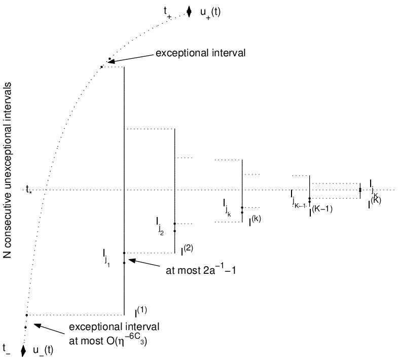 Figure 1
Peer Reviews
No public reviews on file for this paper yet. If you reviewed it on a platform where reviews are public (OpenReview, ICLR, NeurIPS, ICML), you can paste yours below so the community can read it here.
Videos
No videos yet. Explain this paper in a talk, walkthrough, or lecture? Add one.
Global well-posedness and scattering for the energy-critical, defocusing Hartree equation for radial data
Changxing Miao, Guixiang Xu, and Lifeng Zhao
Institute of Applied Physics and Computational Mathematics
P. O. Box 8009, Beijing, China, 100088
([email protected], [email protected], [email protected] )
Abstract
We consider the defocusing, -critical Hartree equation for the radial data in all dimensions . We show the global well-posedness and scattering results in the energy space. The new ingredient in this paper is that we first take advantage of the term \displaystyle-\int_{I}\int_{|x|\leq A|I|^{1/2}}|u|^{2}\Delta\Big{(}\frac{1}{|x|}\Big{)}dxdt in the localized Morawetz identity to rule out the possibility of energy concentration, instead of the classical Morawetz estimate dependent of the nonlinearity.
**Key Words: Hartree equation, Global well-posedness, Scattering, Morawetz estimate.
** **AMS Classification: 35Q40, 35Q55, 47J35. **
1 Introduction
In this paper, we study the Cauchy problem for the Hartree equation
[TABLE]
Here f(u)=\big{(}V*|u|^{2}\big{)}u is a nonlinear function of Hartree type for , where denotes the convolution in . In practice, we use the integral formula of
[TABLE]
where .
If the solution of has sufficient smoothness and decay at infinity, it satisfies two conservation laws :
[TABLE]
As explained in [6], the energy is also conserved for the energy solutions .
From the viewpoint of the fractional integral, we rewrite the equation as
[TABLE]
For dimension , the exponent is the unique exponent which is energy critical in the sense that the natural scale transformation
[TABLE]
leaves the energy invariant, in other words, the energy is a dimensionless quantity.
The Cauchy problem of the Hartree equation has been intensively studied ([4-10], [15, 16, 18, 19]. With regard to the global well-posedness and scattering results, they all dealt with the -subcritical case \big{(}2<\gamma<\min(4,n)\big{)} in the energy space or some weighted spaces. In [16], we obtained the small data scattering result for the -critical case in the energy space. For the large initial data for the -critical case \big{(}\gamma=4,n\geq 5\big{)} in the energy space , the argument in [16] can not yield the global well-posedness, even with the conservation of the energy , because the time of existence given by the local theory depends on the profile of the data as well as on the energy.
Concerning the -subcritical case \big{(}2<\gamma<\min(4,n)\big{)}, using the method of Morawetz and Strauss [17], J. Ginibre and G. Velo [6] developed the scattering theory in the energy space, where they exploited the properties of and obtain the usual Morawetz estimate
[TABLE]
Later, K. Nakanishi [18] exploited the properties of and used a certain related Sobolev-type inequality to obtain a new Morawetz estimate
[TABLE]
which was independent of the nonlinearity.
In this paper, we deal with the Cauchy problem of the Hartree equation with the large data for the -critical case \big{(}\gamma=4,n\geq 5\big{)}. Inspired by the approach of Bourgain [1] and Tao [22] in the case of the -critical Schrödinger equation with the local nonlinear term, we obtain the global well-posedness and scattering results for the Hartree equation for the large radial data in . The new ingredient is that we take advantage of the following localized estimate for the first time
[TABLE]
to rule out the possibility of energy concentration, instead of the classical Morawetz estimate
[TABLE]
due to the nonlinear term .
Our main result is the following global well-posedness result in the energy space.
Theorem 1.1**.**
Let , and be radial. then there exists a unique global solution to
[TABLE]
where and on each compact time interval , we have
[TABLE]
As the right hand side of is independent of , we can obtain the global spacetime estimate. As a direct consequence of the global estimate, we have scattering, asymptotic completeness, and uniform regularity.
Corollary 1.1**.**
Let be radial and have finite energy. Then there exists finite energy solutions to the free Schrödinger equation such that
[TABLE]
Furthermore, the maps are homeomorphisms from to . Finally, if for some , then for all time , and one has the uniform bounds
[TABLE]
The paper is organized as follows.
In Section , we introduce notations and the basic estimates; In Section , we derive the local mass conservation and Morawetz inequality; In Section , we discuss the local theory for ; In Section , we obtain the perturbation theory; Finally, we prove the main theorem in Section .
2 Notations and basic estimates
We will often use the notations and to denote the estimate for some . The derivative operator refers to the space variable only. We also occasionally use subscripts to denote the spatial derivatives and use the summation convention over repeated indices.
We define , , ; For we denote by the dual exponent, that is, .
For any time interval , we use to denote the mixed spacetime Lebesgue norm
[TABLE]
with the usual modifications when . When , we abbreviate by .
We use to denote the free group generated by the free Schrödinger equation . It can commute with derivatives, and obeys the inequality
[TABLE]
for , .
We say that a pair is admissible if
[TABLE]
and
[TABLE]
For a spacetime slab , we define the Strichartz norm by
[TABLE]
and define by
[TABLE]
When , the spaces \big{(}\dot{S}^{0}(I),\|\cdot\|_{\dot{S}^{0}(I)}\big{)} and \big{(}\dot{S}^{1}(I),\|\cdot\|_{\dot{S}^{1}(I)}\big{)} are Banach spaces, respectively.
Based on the above notations, we have the following *Strichartz
- inequalities
Lemma 2.1**.**
[11]**, [21] Let be an solution to the Schrödinger equation . Then
[TABLE]
for any and any admissible pairs . The implicit constant is independent of the choice of interval .
From Sobolev embedding, we have
Lemma 2.2**.**
For any function on , we have
[TABLE]
where all spacetime norms are on .
For convenience, we introduce two abbreviated notations. For a time interval , we denote
[TABLE]
Lemma 2.3**.**
Let \displaystyle f(u)(t,x)=\big{(}uV*|u|^{2}\big{)}(t,x), where . For any time interval and , we have
[TABLE]
**Proof: ** By Strichartz estimates, Hardy-Littlewood-Sobolev inequality and Hölder inequality, we have
[TABLE]
3 Local mass conservation and Morawetz inequality
In this section, we will prove two useful estimates. One is a local mass conservation estimate and the other is a Morawetz inequality, which appears in Morawetz identity. The local mass conservation estimate is used to control the flow of mass through a region of space, and the Morawetz inequality is used to prevent concentration.
3.1 Local mass conservation
We recall a local mass conservation law that has appeared in [1], [13] and [22]. For completeness, we give the sketch of the proof. Let be a bump function supported on the ball that equals on the ball . Observe that if is a finite energy solution of , then
[TABLE]
We define
[TABLE]
Differentiating the above quantity with respect to time, we obtain by the integration by parts
[TABLE]
hence, we have
[TABLE]
This implies that if the local mass is large for some time , then it can also be shown to be similarly large for nearly time , by increasing the radius if necessary to reduce the rate of change of the mass.
On the other hand, from Sobolev and Hölder inequalities, we have
[TABLE]
This gives the control of mass in small volumes.
3.2 A Morawetz inequality
To prevent the concentration of the energy, we need a Morawetz estimate. The Morawetz estimate is based on some integral identity derived by variation of the lagrangian.
We define by
[TABLE]
is the lagrangian density associated to the equation .
From the definition of the variation of the functional , we have
[TABLE]
Using this identity together with and , we obtain the following formula:
[TABLE]
As a consequence of the above dilation identity, we have the following Morawetz estimate, which plays an important role in our proof.
Proposition 3.1** (Morawetz estimate).**
Let u be a solution to on a spacetime slab . Then for any , we have
[TABLE]
where \Omega=\big{\{}(x,y)\in\mathbb{R}^{n}\times\mathbb{R}^{n};|x|\leq A|I|^{1/2};|y|\leq A|I|^{1/2}\big{\}}.
Remark 3.1**.**
Since
[TABLE]
we have
[TABLE]
Proof: We define , then
[TABLE]
and
[TABLE]
where we use the symmetry of and . Let and let be a bump function adapted to the ball which equals 1 on the ball . We set .
For , we have
[TABLE]
and for , we have bounds
[TABLE]
Thus we have
[TABLE]
where ,
[TABLE]
Meanwhile
[TABLE]
[TABLE]
Moreover, from Sobolev and Hölder inequalities, we have
[TABLE]
So if we integrate by parts on a time interval I and take , we obtain
[TABLE]
for . The proof is completed.
4 Local theory
In this section, we develop a local well-posedness and blow-up criterion for the -critical Hartree equation. First, we have
Proposition 4.1** (Local well-posedness).**
Let , and be a compact time interval that contains such that
[TABLE]
for a sufficiently small absolute constant . Then there exists a unique strong solution to on such that
[TABLE]
**Proof: ** The proof of this proposition is standard and based on the contraction mapping arguments. We define the solution map to be
[TABLE]
then is a map from
[TABLE]
with the metric
[TABLE]
onto itself because
[TABLE]
[TABLE]
It suffices to prove is a contraction map. Let , , then
[TABLE]
By Lemma 2.3, we have
[TABLE]
In the same way, we have
[TABLE]
as long as is chosen sufficiently small. Then the contraction mapping theorem implies the existence of the unique solution to (1.4) on I.
Next, we give the blow-up criterion of the solutions for . The usual form is similar to those in [2], [12], which is in the form of a maximal interval of existence. For convenience, we obtain
Proposition 4.2** (Blow-up criterion).**
Let , and let be a strong solution to on the slab such that
[TABLE]
Then there exists such that the solution extends to a strong solution to on the slab .
**Proof: ** By the absolute continuity of integrals, there exists a , such that
[TABLE]
then by Lemma 2.3, we have
[TABLE]
therefore
[TABLE]
Now we write
[TABLE]
then
[TABLE]
By the absolute continuity of integrals again, there exists a , such that
[TABLE]
Thus we may apply Proposition 4.1 on the interval to complete the proof.
In other words, this lemma asserts that if is the maximal interval of existence and , then
[TABLE]
5 Perturbation result
In this section, we obtain the perturbation for Hartree equation, which shows that the solution can not be large if the linear part of the solution is not large. This is an analogue of Lemma in [22], and later, Killip, Visan and Zhang [13] gave the similar perturbation result for the Schrödinger equation with the quadric potentials.
Lemma 5.1** (Perturbation lemma).**
Let be a solution to on such that
[TABLE]
where is sufficiently small constant depending on the norm of the initial data, then
[TABLE]
where for .
**Proof: ** From Strichartz estimate and Lemma 2.3, we obtain
[TABLE]
If is sufficiently small, we have the first claim
[TABLE]
As for the second claim, we give the proof for , the case is similar. Using Strichartz estimate and Lemma 2.3 again, we have
[TABLE]
therefore, the second claim follows by the triangle inequality and choosing sufficiently small.
6 Global well-posedness
In this section, we give the proof of Theorem 1.1. The new ingredient is that we first take advantage of the the estimate of the term in the localized Morawetz identity to rule out the possibility of energy concentration, which is independent of the nonlinear term. For the Schrödinger equation, Tao [22] used the classical Morawetz estimate, which depends on the nonlinearity, to prevent the concentration.
For readability, we first take some constants
[TABLE]
which come from several constraints in the rest of this section. All implicit constants in this section are permitted to depend on the dimension and the energy.
Fix , , . We may assume that the energy is large, , otherwise the claim follows from the small energy theory [16]. From the boundedness of energy and Sobolev embedding, we can obtain
[TABLE]
for all .
Assume that the solution already exists on . By Lemma 4.2, it suffices to obtain a priori estimate
[TABLE]
where is independent of , .
We may assume that
[TABLE]
otherwise it is trivial. We divide into subintervals for some such that
[TABLE]
where is a small constant depending on the dimension and the energy. As a consequence, it suffices to estimate the number .
Now let . By Sobolev embedding and Strichartz estimates, we have
[TABLE]
We adapt the following definition of Tao [22].
Definition 6.1**.**
We call exceptional if
[TABLE]
for at least one sign . Otherwise, we call unexceptional.
From , we obtain the upper bound on the number of exceptional intervals, . We may assume that there exist unexceptional intervals, otherwise the claim would follow from this bound and . Therefore, it suffices to compute the number of unexceptional intervals.
We first prove the existence of a bubble of mass concentration in each unexceptional interval.
Proposition 6.1** (Existence of a bubble).**
Let be an unexceptional interval. Then there exists such that
[TABLE]
for all .
**Proof: ** By time translation invariance and scale invariance, we may assume that . We subdivide further into and . By and the pigeonhole principle and time reflection symmetry if necessary, we may assume that
[TABLE]
Thus by Lemma 5.1, we have
[TABLE]
By Duhamel formula, we have
[TABLE]
Since is unexceptional interval, we have
[TABLE]
On the other hand, by , Lemma 2.2 , Lemma 2.3 and Lemma 5.1, we have
[TABLE]
Thus the triangle inequality implies that
[TABLE]
provided is chosen sufficiently small. Hence, if we define
[TABLE]
then we have
[TABLE]
Next, we estimate the upper bound on . We have by and the triangle inequality
[TABLE]
where we use Strichartz estimate, and Lemma 5.1.
We shall need some additional regularity control on . For any , let denote the translation of by , i.e. .
Lemma 6.1**.**
Let be a bump function supported on the ball of total mass one, and define
[TABLE]
then we have
[TABLE]
**Proof: ** By the chain rule, Hölder inequality and Sobolev embedding, we have
[TABLE]
it follows by
[TABLE]
From and interpolation, we have
[TABLE]
From the fundamental theorem of calculus, we have
[TABLE]
This implies
[TABLE]
Hence from Hölder inequality, we obtain
[TABLE]
This completes the proof of Lemma.
Now we return to the proof of Proposition 6.1. By Lemma 6.1 and , we have
[TABLE]
On the other hand, by Hölder inequality, Young inequalities and , we have
[TABLE]
Interpolating with gives
[TABLE]
Thus there exists such that
[TABLE]
Hence, by Cauchy-Schwarz inequality, we have
[TABLE]
that is
[TABLE]
Observe that also holds for . If we take and choose sufficiently small, we have
[TABLE]
for all .
The last step is to show that this mass concentration holds for . We first show mass concentration for at time [math].
Since is unexceptional interval, by the pigeonhole principle, there is a such that
[TABLE]
and so by Hölder inequality,
[TABLE]
From , we have
[TABLE]
Recall that . Combing and with the triangle inequality, we obtain
[TABLE]
Using again, we obtain the result.
Next, we use the radial assumption to show that the bubble of mass concentration must occur at the spatial origin. In the forthcoming paper, we shall use the interaction Morawetz estimate with the frequency localized almost-conservation law to rule out the possibility of the energy concentration at any place and deal with the non-radial data. The corresponding results for the Schrödinger equation with local nonlinearity, please see [3], [20] and [23].
Corollary 6.1** (Bubble at the origin).**
Let be an unexceptional interval. Then
[TABLE]
for all .
**Proof: ** If in Proposition 6.1 is within of the origin, then the result follows immediately. Otherwise by the radial assumption, there would be at least
[TABLE]
many distinct balls each containing at least amount of mass. By Hölder inequality, this implies
[TABLE]
that is
[TABLE]
Because for , this contradicts the boundedness on the energy of . This completes the proof.
Next, we use Proposition 3.1 to show that if there are many unexceptional intervals, they must form a cascade and must concentrate at some time .
Corollary 6.2**.**
Assume that the solution is spherically symmetric. For any interval and be a union of consecutive unexceptional intervals . Then
[TABLE]
and moreover, there exists a such that
[TABLE]
**Proof: ** For any unexceptional interval , from Hölder inequality and Corollary 6.1, we have
[TABLE]
therefore
[TABLE]
We integrate this over each unexceptional interval and sum over ,
[TABLE]
The second claim follows from the first and the fact that
[TABLE]
This completes the proof.
Proposition 6.2** (Interval cascade).**
Let be an interval tiled by finitely many intervals . Suppose that for any continuous family \big{\{}I_{j}:j\in\mathcal{J}\big{\}} of the unexceptional intervals, there exists such that
[TABLE]
for some small . Then there exist distinct indices such that
[TABLE]
and for any ,
[TABLE]
hold for .
**Proof: ** Here we use an algorithm in [1] and [22] to assign a generation to each .
By hypothesis, contains at least one interval of length . All intervals with length larger than belong to the first generation. By the total measure, we see that there are at most intervals in the first generation. Removing there intervals from leaves at most gaps, which are tiled by intervals .
By and the contradiction argument, we know that there is not gap with length larger than .
We now apply this argument recursively to all gaps generated by the previous iteration until every has been labeled with a generation number.
Each iteration of the algorithm removes at most many intervals and produces at most gaps. Suppose that there are consecutive unexceptional intervals initially, and we perform at most times iterations. Then the number obeys
[TABLE]
which leads to the claim .
Let be the interval obtained after iterations and be any interval in . For , let be the -generation gap which contains the , and assign the be any ith-generation interval which is contained in (see Figure ). By the construction, for any , we have
[TABLE]
for all .
Proposition 6.3** (Energy non-evacuation).**
Let be a disjoint family of unexceptional intervals obeying
[TABLE]
and for any ,
[TABLE]
hold for . Then
[TABLE]
**Proof: ** By Corollary 6.1,
[TABLE]
for all . By , we have
[TABLE]
On the other hand, from , we have
[TABLE]
Define
[TABLE]
then we have
[TABLE]
By Hölder inequality, we have
[TABLE]
Choosing , then we obtain by
[TABLE]
Hence the annuli associated to are disjoint. The number of such annuli is .
Therefore from , we obtain
[TABLE]
That is
[TABLE]
We now return to the proof of Theorem 1.1. As explained at the beginning of this section, it suffices to bound the number of the unexceptional intervals.
Note that the number of exceptional interval is at most . We first bound the number of unexceptional intervals that can occur consecutively.
Let us denote the union of these consecutive unexceptional intervals by . By Corollary 6.2, the hypotheses of Proposition 6.2 are satisfied with and so we can find a cascade of intervals and they satisfied the hypotheses of Proposition 6.3. The bound on implies the bound on , namely,
[TABLE]
At last, since there are at most exceptional intervals, the total number of intervals is
[TABLE]
This completes the proof of Theorem 1.1.
Acknowledgements: The authors were partly supported by the NNSF of China. G. Xu wish to thank Xiaoyi Zhang for providing the paper [13] and some discussions.
The reference list from the paper itself. Each links out to its DOI / PubMed record.
- 1[1] J. Bourgain, Scattering in the energy space and below for 3D NLS. J. Anal. Math. 75(1998), 267-297.
- 2[2] T. Cazenave, Semilinear Schrödinger equations. Courant Lecture Notes in Mathematics, vol. 10. New York: New York University Courant Institute of Mathematical Sciences, 2003.
- 3[3] J. Colliander, M. Keel, G. Staffilani, H. Takaoka, and T. Tao, Global well-posedness and scattering for the energy-cirtical nonlinear Schrödinger equation in ℝ 3 superscript ℝ 3 \mathbb{R}^{3} . to appear Ann. of Math..
- 4[4] J. Ginibre and T. Ozawa, Long range scattering for nonlinear Schrödinger and Hartree equations in space dimension n ≥ 2 . 𝑛 2 n\geq 2. Comm. Math. Phys., 151(1993), 619-645.
- 5[5] J. Ginibre and G. Velo, On a class of nonlinear Schrödinger equations with nonlocal interactions, Math. Z., 170(1980), 109-136.
- 6[6] J. Ginibre and G. Velo, Scattering theory in the energy space for a class of Hartree equations, Nonlinear wave equations (Providence, RI, 1998), 29-60, Contemp. Math., 263, Amer. Math. Soc., Providence, RI, 2000.
- 7[7] J. Ginibre and G. Velo, Long range scattering and modified wave operators for some Hartree type equations. Rev. Math. Phys., 12, No. 3, 361-429 (2000).
- 8[8] J. Ginibre and G. Velo, Long range scattering and modified wave operators for some Hartree type equations II. Ann. Henri Poincaré 1, No.4, 753-800 (2000).