Sum-over-states vs quasiparticle pictures of coherent correlation spectroscopy of excitons in semiconductors; femtosecond analogues of multidimensional NMR
Shaul Mukamel, Rafal Oszwaldowski, Darius Abramavicius

TL;DR
This paper compares the sum-over-states and quasiparticle approaches to understanding 2D correlation spectroscopy of excitons in semiconductors, providing a formal connection between the two methods using Green's functions.
Contribution
It derives Green's function expressions linking the sum-over-states and quasiparticle pictures for 2DCS signals in semiconductors, clarifying their relationship.
Findings
Established formal connection between the two theoretical pictures
Linked the approaches to Frenkel and vibrational excitons
Provided Green's function framework for 2DCS analysis
Abstract
Two-dimensional correlation spectroscopy (2DCS) based on the nonlinear optical response of excitons to sequences of ultrafast pulses, has the potential to provide some unique insights into carrier dynamics in semiconductors. The most prominent feature of 2DCS, cross peaks, can best be understood using a sum-over-states picture involving the many-body eigenstates. However, the optical response of semiconductors is usually calculated by solving truncated equations of motion for dynamical variables, which result in a quasiparticle picture. In this work we derive Green's function expressions for the four wave mixing signals generated in various phase-matching directions and use them to establish the connection between the two pictures. The formal connection with Frenkel excitons (hard-core bosons) and vibrational excitons (soft-core bosons) is pointed out.
Click any figure to enlarge with its caption.
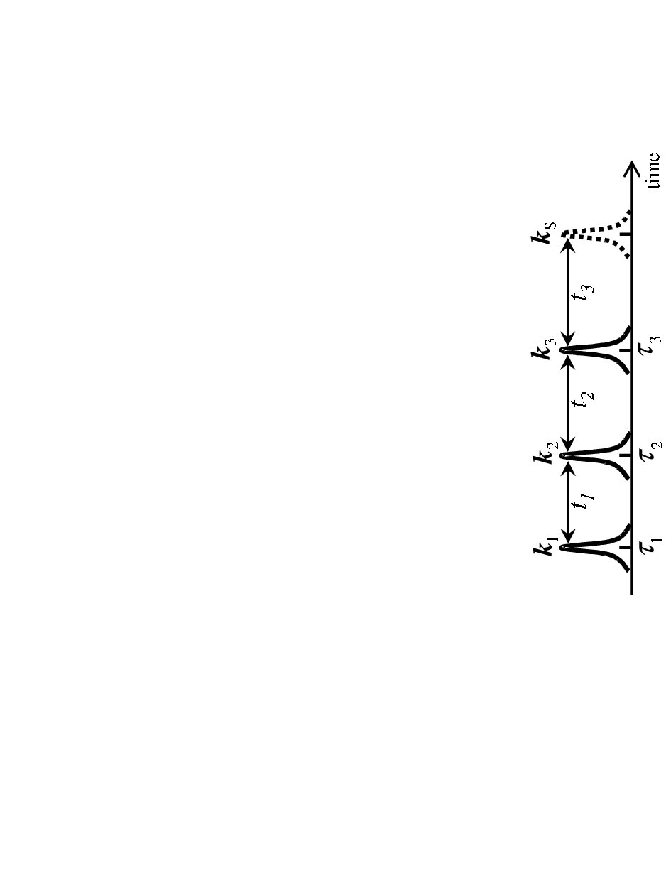 Figure 1
Peer Reviews
No public reviews on file for this paper yet. If you reviewed it on a platform where reviews are public (OpenReview, ICLR, NeurIPS, ICML), you can paste yours below so the community can read it here.
Videos
No videos yet. Explain this paper in a talk, walkthrough, or lecture? Add one.
Sum-over-states vs quasiparticle pictures of
coherent correlation spectroscopy of excitons in semiconductors; femtosecond analogues of multidimensional NMR
Shaul Mukamel, Rafal Oszwaldowski, Darius Abramavicius
Chemistry Department, University of California, Irvine, CA 92697-2025, United States
Abstract
Two-dimensional correlation spectroscopy (2DCS) based on the nonlinear optical response of excitons to sequences of ultrafast pulses, has the potential to provide some unique insights into carrier dynamics in semiconductors. The most prominent feature of 2DCS, cross peaks, can best be understood using a sum-over-states picture involving the many-body eigenstates. However, the optical response of semiconductors is usually calculated by solving truncated equations of motion for dynamical variables, which result in a quasiparticle picture. In this work we derive Green’s function expressions for the four wave mixing signals generated in various phase-matching directions and use them to establish the connection between the two pictures. The formal connection with Frenkel excitons (hard-core bosons) and vibrational excitons (soft-core bosons) is pointed out.
pacs:
78.47.+p,71.35.-y
I Introduction
Exciton models are widely used to describe the linear and nonlinear optical properties of many types of systems, including semiconductor nanostructures (quantum wells, dots and wires), molecular aggregates and crystals,Davydov (1962); Mukamel (1993); Chernyak et al. (1998a) as well as vibrations in proteins.Zhuang et al. (2005); Mukamel and Abramavicius (2004) In semiconductors, nonlinear optical experiments reveal a wealth of interesting phenomena.Chemla and Shah (2001); Kaindl et al. (2001); Shih et al. (2005); Shah (1999); Meier et al. (2006) For instance, such experiments provide information about many-exciton states such as biexcitons, their interactions, relaxation and dissociation.Chemla (2001); Adachi et al. (2004); Rice et al. (2005); Danckwerts et al. (2006)
The introduction of multidimensional techniques had revolutionized NMR in the seventiesAue et al. (1976) and established it as a powerful tool for studying complex systems and identifying specific structural and dynamical correlations.Ernst et al. (1989) In such experiments the system is subjected to a sequence of well separated pulses. Correlation plots of the signals vs. two (or more) time delay periods then provide multidimensional spectroscopic windows into the system. The correlated dynamics of spins carefully prepared by the pulse sequence is very sensitive to their interactions. Analysis of these correlation plots then provides a powerful probe for molecular geometries and dynamical correlations. These techniques were recently extended to the infrared and the visible regime and were shown to be very useful for Frenkel excitons in molecular systems.Mukamel (2000); Tanimura and Mukamel (1993); Mukamel and Abramavicius (2004); Zhang et al. (1999) There are some differences between the optical and the NMR techniques. NMR uses strong saturating fields whereas optical pulses are most effective in the weak field regime. NMR signals are essentially isotropic in space whereas coherent optical signals are generated in well defined (phase-matching) directions. These differences were explored in detail in Refs. Scheurer and Mukamel, 2002a; Scheurer and Mukamel, 2001, 2002b. Nevertheless the NMR and optical techniques are conceptually similar and many ideas of pulse sequences developed in NMR may be adopted in the optical regime, where the millisecond NMR time-scale is pushed to the femtosecond regime. The same ideas may be extended to study interband and intersuband excitations in semiconductors.Yang et al. (2006); Kuznetsova et al. (2007); Erementchouk et al. (2006); Li et al. (2006); Borca et al. (2005) Multidimensional analysis of the nonlinear optical response of semiconductors to sequences of femtosecond pulses could provide a novel probe for many-body interactions. In a recent workYang et al. (2006) on semiconductor Quantum Wells, 2D correlation spectra from three 3rd order optical techniques have been calculated. The unique character of 2D spectroscopy allowed to easily recognize and classify features due to different types of biexcitons. Such features are sometimes difficult to separate in the usual one-dimensional mode of displaying non-linear spectra, due to the strong line broadening and the highly congested exciton spectra.
Two types of approaches have been traditionally used towards modeling the nonlinear optical response of excitonic systems. The first is based on the many-body eigenstates obtained by exact diagonalization of the Hamiltonian.Mukamel (1995) Sum-over-states (SOS) expressions can then be derived for the nonlinear response functions and optical signals. This method is practical in many applications to electronic and vibrational Frenkel excitons in moleculesBrixner et al. (2005); Fang et al. (2004); Abramavicius et al. (2004) and allows clear identification and classification of possible single- and multi-photon resonances. Calculating the eigenstates is a serious computational bottleneck in extended structures. For an site tight-binding Frenkel-exciton model the number of single and two-exciton states scales as and respectively. For Wannier excitons in semiconductors these scalings are and , making the simulations prohibitively expensive. This is why the approach is not widely used for electron-hole excitations in semiconductors. Instead, one adopts a second strategy, which describes the response in terms of quasiparticles (QP), and the many-particle eigenstates are never calculated. Spano and Mukamel (1989); Leegwater and Mukamel (1992); Mukamel (1995); Chernyak and Mukamel (1996); Spano and Mukamel (1991); Mukamel (1993) Calculations are performed by solving equations of motion for microscopic coherences, which are coupled to other dynamical variables. Even for a simple system such as a single semiconductor quantum well, solving the equations numerically to create a 2D map of a nonlinear response function is computationally expensive,Yang et al. (2006) since these equations must be solved repeatedly for different pulse delays. Only after obtaining the optical signal on a 2D time grid, a Fourier transform can be performed to get the 2DCS. Apart from direct, numerical solutions of equations of motion Koch et al. (1999); Weiser et al. (2000) there exist other theoretical approaches to exciton correlation effects, such as memory kernel representation Östreich et al. (1995); Axt et al. (2001) or Coupled Cluster Expansion for doped semiconductors.Primozich et al. (2000); Shahbazyan et al. (2000)
In this paper we derive closed expressions for 2DCS of semiconductors by solving the Nonlinear Exciton Equations (NEE)Axt and Mukamel (1998); Chernyak et al. (1998a) for the third order response. Both time-ordered and non-ordered forms of the response function which represent time and frequency domain techniques, respectively, are derived. Our QP expressions for the response are given in terms of the single exciton Green’s function and the exciton scattering matrix. The SOS response functions, in contrast, are expressed in terms of many-exciton eigenstates. Even though the response functions calculated using both techniques must be identical, the relation between the two pictures is not obvious. The expressions look very different and it is not possible to see their equivalence by a simple inspection. The SOS expressions contain large terms, which grow with system size and have opposite signs, thus they almost cancel. This complicates their numerical implementation. In contrast these cancellations are built-in from the outset in the QP approach, which uses a harmonic reference system. The nonlinearities are then attributed to exciton-exciton scattering which is absent in the harmonic reference system. The second goal of this paper is to show precisely how the two pictures of many-body correlations are connected. We write down the SOS expressions using the Keldysh loop and then derive the QP expressions directly from the SOS ones. This provides a time-domain interpretation for the interference effects. The SOS and the QP expressions provide complementary views into the origin of features seen in 2D spectrograms.
In Sec. II we present the SOS expressions for the third order response obtained from time-dependent perturbation theory. Their QP counterparts are derived in Sec. III. We use the method developed in Refs. Chernyak and Mukamel, 1996; Chernyak et al., 1998a to transform the Hamiltonian to a form typical for interacting oscillators. The starting many-electron Hamiltonian can be written in an ab-initio,Oszwałdowski et al. (2005) tight-binding Sieh et al. (1999a) or a basis. One of the key results of this paper, i.e., the equivalence of the SOS and QP pictures is proven in Sec. IV. In Sec. V we derive closed expressions for 2D correlation signals. The QP approach provides a unified description for electron-hole excitations in semiconductors as well as to Frenkel excitons in molecular aggregates (Paulions) and anharmonic vibrations (bosons), which are described by the same general Hamiltonian. QP formulae for nonlinear response have been derived previously along similar lines for Frenkel excitons. This connection is shown in Appendix F. In the last Section (VI) we discuss the results.
II Sum-over-states expressions for the time-ordered nonlinear response
We consider a 4 wave-mixing experiment performed with three femtosecond laser pulses (Fig. 1). The optical electric field is:
[TABLE]
[TABLE]
[TABLE]
The -th pulse is centered at , has an envelope , carrier frequency , and wavevector . () denotes the positive (negative) frequency part of the field, and . The induced polarization in the system is recorded as a function of time-delays between pulses.
Assuming the dipole interaction with the optical field , where is the dipole operator, the third-order contribution to the system’s polarization can be written as
[TABLE]
where the response function , which connects the induced polarization with the laser field envelopes, is given by (throughout this paper we set ):
[TABLE]
We shall use double-sided Feynman diagrams to represent the time ordering of various interactions.Mukamel (2005) The four terms in Eq. (5) are represented by diagrams a, b, c, d shown on Figure 2. These diagrams should be read starting at the bottom left and proceeding along the loop, clockwise, as indicated by the arrows. The variables are ordered on the Keldysh-Schwinger loop, but not necessarily in real (physical) time. in diagrams (a) and (d) are also ordered in real time. This is not the case for diagrams (b) and (c): in (b) can come either before or after and , whereas in (c) can come either before or after and .
If the eigenstates and eigenvalues of the system are known, Eq. (5) may be expanded in terms of the corresponding matrix elements:
[TABLE]
So far we considered a general multilevel system. We next turn to the response of excitons, where the energy levels form manifolds, classified by the number of excitons: the ground state , single exciton , two-exciton (or biexciton), etc. (Fig. 3). We shall assume that the dipole operator can only create and annihilate a single exciton at a time. Only the single and the two-exciton states then contribute to the third order signals. We further partition the dipole operator as , where is the positive frequency part which induces upward to and to transitions, while its Hermitian conjugate (the negative frequency part) induces the opposite transitions. We thus write
[TABLE]
Invoking the rotating-wave approximation (RWA), we neglect all terms where at least one of the transitions is not in resonance with one of the incident carrier frequencies. The system-field interaction term then becomes
[TABLE]
Each correlation function in Eq. (5) will split into terms upon substituting Assuming that the system is initially in the ground state, only two of these contributions are non-zero
[TABLE]
Substitution of Eq. (7) into Eq. (5) gives
[TABLE]
The four terms represented by the diagrams in Fig. 4 were obtained by taking for the last interaction, gives the complex conjugates. Hereafter left/right direction of the arrows corresponds to in Eq.(8). Note that time-reversal symmetry implies . If the pulse envelopes are much shorter than their delays, the system is forced to interact sequentially first with pulse , then and finally . This means that in the integral of Eq. (4) one must replace with one of the , depending on the time-ordering of the integration variables in real (physical) time. We note that the first and the second terms in Eq. (8) impose a full time ordering of the integration variables while the third and the fourth terms do not. Term (b) is only partially time ordered. Depending on the position of relative to the sequence, the diagram can be separated into three fully time ordered terms: , or . Formally we do that by separating the product of step functions as follows:
[TABLE]
Using this relation, diagram (b) of Fig. 4 is split into (b3), (b2) and (b1) as shown in the first line of Fig. 5. The interactions on the l.h.s. of this diagrammatic equation are ordered on the loop. On the other hand, the arrows in the open, double-sided diagrams on the r.h.s. are ordered in real (physical) time. All diagrams on the r.h.s. are obtained from (b) by moving the arrows while preserving their order along the loop (but not in physical time!). Similarly we write for term (c)
[TABLE]
and the diagram is split into (c2), (c3), (c1). can now be recast in the fully time-ordered form
[TABLE]
The labels on the right correspond to the various diagrams shown in Figs. (4) and (5).
Once split into fully time-ordered contributions, it is convenient to change the integration variables in Eq. (4) from that label the actual interaction times with the fields, to the three delays between successive interactions. Note that the correlation functions are invariant to time translation . Eq. (4) thus assumes the form
[TABLE]
where In the impulsive limit, where all pulses are shorter than all system’s response time scales, we can substitute Eqs. (1)-(3) in Eq. (10) and eliminate the time integrations. This gives
[TABLE]
The polarization is created along 8 possible directions with
[TABLE]
where
[TABLE]
vanishes for the assumed dipole selection rules in our model. Since , we are left with three independent combinations , , :
[TABLE]
We can classify the diagrams in Fig. 5 according to the directions of the arrows: arrow pointing to the right (left) represents (), arrows are read from the bottom up on either side. We obtain for (Fig. 6)
[TABLE]
For the technique we similarly have (Fig. 7):
[TABLE]
Finally is given by (Fig. 8):
[TABLE]
Each term is labelled according to Eq. (9). Eqs. (13-15) can be used to express the third order SOS response in terms of transition dipoles, system frequencies and dephasing rates (see App. E and Sec. V).
In the next section we employ the EOM approach to derive the alternative QP expressions for these signals. These will then be connected with the current SOS expressions in Section IV.
III Quasiparticle expressions for Wannier excitons in semiconductors
Interband transitions in semiconductors may be described by the two-band many-electron Hamiltonian:Axt and Mukamel (1998); Haug and Koch (2004)
[TABLE]
with the single-particle part
[TABLE]
where create electrons and create holes. The Coulomb interaction is:
[TABLE]
while
[TABLE]
is the dipole interaction with light, and the optical electric field will be treated as a scalar for simplicity. can describe both bulk and low-dimensional semiconductor systems. All the steps in this Section are independent of the single-electron basis used. would be diagonal in the basis of the system’s single-particle eigenstates, i.e., . In this paper we focus on the coherent response and we neglect coupling with phonons, which would result in additional, relevant dynamical variables and new contributions to the response function. Chernyak et al. (1998a); Mukamel (1993) The SOS and QP pictures should be equivalent also when dephasing is included. In that case, however, the theory becomes more complicated. For the sake of simplicity and transparency we restrict the following analysis to the coherent response, where we do not include phonons explicitly. Dephasing effects, necessary for a realistic description, will be simply introduced by adding imaginary parts to excitonic frequencies.
To introduce the exciton representation we define electron-hole operators:Chernyak and Mukamel (1996)
[TABLE]
where we have employed shorthand notation for pairs of indices: . Using these operators we construct an effective Hamiltonian (see App. A):
[TABLE]
The Hamiltonians and are equivalent in the single and double excitations subspace, which is relevant for the response to third order in .Mukamel (1995) This transformation from fermion to exciton variables is crucial for our approach, since it allows us to view the electronic degrees of freedom as a system of coupled oscillators. The parameters of the transformed Hamiltonian are given by:
[TABLE]
The commutation relations for the operators can be obtained using the elementary fermion anticommutators: . Within the subspace of and states (i.e., the ground state and single excitations), we get Chernyak and Mukamel (1996)
[TABLE]
where and
[TABLE]
Eqs. (19) and (20) are obtained in a similar way to (17) and (18). Terms with additional pairs (e.g. ) are neglected in (19), because they would introduce corrections higher than to the nonlinear response. Note the symmetry .
Using Eqs. (17) and (19) we obtain the nonlinear exciton equations (see Appendix B) for single-exciton variables :Spano and Mukamel (1991); Mukamel (1993); Chernyak et al. (1998b); Mukamel (2000)
[TABLE]
where is given by
[TABLE]
Here are two-exciton variables. The Heisenberg equations give:
[TABLE]
Calculating the optical response by numerical integration of these equationsSieh et al. (1999b); Yang et al. (2006) is straightforward but numerically expensive. An alternative, more tractable approach, which further provides a better insight into the nature of the response, is to integrate the equations formally using one-exciton Green’s functions and exciton scattering matrix . The scattering matrix depends on quasiparticle statistics through the matrix (Eqs. 49, 50) as well as on exciton-exciton coupling. This results in closed quasiparticle expressions for the 3rd order contributions , and to the response function (for details see Appendix C and Ref. Abramavicius and Mukamel, 2005)
[TABLE]
where etc. and .
The response functions for the other phase-matching directions can be derived along the same lines. We get
[TABLE]
and:
[TABLE]
Just as in the SOS case, time translation symmetry implies that these response functions only depend on the three pulse delays . Eqs. (24-26) will be used next to connect the QP and the SOS pictures.
IV Connecting the sum-over-states and the quasiparticle pictures
We first recast Eqs. (13-15) using Green’s functions (in all expressions , , ):
[TABLE]
Here and represent the retarded and the advanced Green’s function respectively; , and describe the evolution within the ground-state, single-exciton and double-exciton blocks of the Hamiltonian (Eq. 17) respectively. We also set the ground state energy to zero.
Our goal is to show the equivalence of the QP and SOS pictures by deriving Eqs. (24-26) from Eqs. (27-29). To that end we adopt a harmonic reference system of noninteracting quasiparticle and expand the SOS response in anharmonicities. Harmonic oscillators are linear, and their nonlinear response vanishes identically Spano and Mukamel (1989); Kuhn et al. (1996); Mukamel (1993, 1995), as can be easily seen from the Heisenberg equations of motion. This means that the various Liouville space pathways for all nonlinear response function interfere destructively. Exploiting this property in the following derivation, we show that the quasiparticle physical picture has built-in cancellations in the reference harmonic system.
We shall use the Dyson equation for the two particle Green’s function, also known as the Bethe-Salpeter equationLeegwater and Mukamel (1992)
[TABLE]
or in the time domain:
[TABLE]
is taken to be the Green’s function of a doubly excited, harmonic system. It can be factorized into the product of a single-exciton Green’s functions
[TABLE]
The exciton scattering matrix is defined by Eq. (31).
Let us start with the technique and show the equivalence of Eq. (27) to (24). The second and third terms of Eq. (27) (diagrams (c1) and (c3) in Fig. 6) are purely harmonic, independent on the quasiparticle interactions. This is a direct result of the ordering of , whereby the system only evolves in the ground and first excited state. Exciton-exciton interactions influence the evolution only in the second excited manifold. The first term in Eq. (31), i.e. , represents harmonic evolution in the two-exciton manifold. Thus the first term of Eq. (27) with replaced by must cancel the other two terms, because the nonlinear response of a harmonic system vanishes. Substituting the second term from Eq. (31) in Eq. (27) we obtain a single term for :
[TABLE]
The equivalence of the Eqs. (32) and (24) can be directly seen using the diagrams shown in Fig. (9). In these diagrams the scattering matrix is represented by dashed regions. Note that . The QP diagram in Fig. (9) is obtained from the SOS one by changing the integration variables and This completes the derivation of the QP expression for (Eq. 24) starting from the SOS expression (Eq. 27).
can be calculated similarly. By combining Eqs. (28) and (31) the same type of cancellation of harmonic terms yields
[TABLE]
Eq. (33) is identical to Eq. (25) as illustrated in Fig. (10).
We finally turn to , (Eq. 29). Using again the Bethe Salpeter equation (31) and the fact that terms that only depend on must cancel (harmonic reference), we get
[TABLE]
The equivalence of QP (Eq. 26) and SOS (Eq. 29) expressions can be shown as follows: the two terms in Eq. (34) are labeled (SOSa) and (SOSb). The term (SOSb) can further be split into two terms (SOSb1) and (SOSb2), the first corresponding to , the second to (Fig. 11). (SOSb1) is identical to (SOSa), but with opposite sign coming from . Only the second term (SOSb2) remains, and it is equivalent to the (QP) diagram. We thus obtained Eq. (26) from Eq. (34).
V 2D correlation signals
2D signals are displayed as correlation plots obtained by the double Fourier transforms of the various signals.Mukamel (2000) We shall denote the frequencies conjugate to the pulse delay times and by and . Starting with Eq. (11), and deleting some inessential factors, we obtain the induced polarization, which depends parametrically on the delay times , and :
[TABLE]
Specifying the three possible signals by a proper choice of factors we obtain:
[TABLE]
The 2DCS for and is defined as
[TABLE]
For the SOS picture we use the expansions in eigenstates given by Eqs. (59), (60) and (61). The QP expressions for , and are obtained along the lines presented in App. C. Dephasing is introduced phenomenologically by adding a decay rate to the Green’s functions. We thus obtain
[TABLE]
[TABLE]
The Green’s function Fourier transform is defined as [and ]. We have
[TABLE]
Eq. (40) is obtained by transforming to the single-exciton basis and performing the Fourier transform. We also define
[TABLE]
Similarly we obtain for :
[TABLE]
[TABLE]
The 2DCS signal is defined as
[TABLE]
This yields:
[TABLE]
[TABLE]
Both and depend on the single-exciton energies. However, the SOS expressions contain two-exciton eigenenergies () explicitly, while the QP counterparts contain the scattering matrix instead. The equivalence of the two representations has been established in Sec. IV. Eqs. (37-45) constitute our final expressions for the various 2DCS signals. In this form they may be readily used in numerical simulations. The SOS expressions (Eqs. 37, 41 and 44) were recently used to survey the various possible resonances and cross-peaks in 2DCS of semiconductors.Yang et al. (2006)
VI Discussion
The quasiparticle representation is obtained using the Heisenberg equations for the exciton oscillator variables. These equations form an infinite hierarchy involving successively higher numbers of excitons.Abramavicius and Mukamel (2006a); Chernyak et al. (1998a) The hierarchy may be truncated, depending on the observable of interest. For instance, the absorption originates from single-exciton creation/annihilation. Only single-exciton variables should then be considered, and exciton-exciton interaction terms may be neglected. The nonlinear response depends on the exciton interactions, thus single- and double-exciton variables need to be treated explicitly. The two coupled NEE equations (21, 23) describe the third order response. These equations are exact in the absence of dephasing. When dephasing is included by adding linear coupling to a phonon bath, two additional variables and must be included in the NEE to describe the third order response. Chernyak et al. (1998a) Without dephasing these may be factorized as and . We then recover the coherent limit considered in this article. For some techniques the present equations provide a good approximation even in the presence of dephasing. describes incoherent exciton transport and is only relevant during , while is generated during . It describes the optical coherence between one-exciton and two-exciton manifolds, which are represented by and .
The quasiparticle approach avoids the explicit calculation of multiple exciton states: their influence is represented by the scattering matrix, which can be calculated provided the exciton interactions are known. We have shown how the quasiparticle expressions for the various third order techniques, ordinarily derived by solving equations of motion, can be obtained directly from the sum-over-states expressions by employing the Bethe-Salpether equation. These expressions explicitly contain the two-exciton Green’s functions and have many interfering terms with large cancellations,Spano and Mukamel (1989) which complicate their numerical implementation. In the QP picture, on the other hand, these interference effects are built-in, considerably simplifying the expressions for the nonlinear response.Spano and Mukamel (1991)
The interpretation of 2DCS signals using the SOS expressions is straightforward.Yang et al. (2006) In the technique one-exciton coherences are observed during , and the coherences between excitons and biexcitons are observed during . Thus the 2DCS shows peaks along and corresponding to these resonances. shows biexciton resonances along the axis, this technique is known in NMR as double-quantum coherence. We have established the connection between the SOS and the QP pictures by using time-ordering on the Keldysh-Schwinger loop, which only maintains partial time ordering in real (physical) time.
The Hamiltonian (Eq. 17) can describe several microscopic models other than the Wannier excitons considered here (). Vibrational excitations (soft-core bosons) and Frenkel excitons (hard-core bosons, Paulions) in molecules can be mapped into the same model. Zhang et al. (1999); Abramavicius and Mukamel (2006a); Kuhn et al. (1996) The equations of motion for these other systems are similar, but not identical, because of the different commutation relations (QP statistics). Eq. (19) provides a unified description for all of these systems, by specifying the proper commutation rules:Chernyak and Mukamel (1996); Chernyak et al. (1998a) for bosons and for Paulions . These expressions for may be substituted into our final expressions for the response functions, where they only affect the exciton scattering matrix, which in the frequency domain reads (App. D)
[TABLE]
where is given in Eq. (22), is the free two–exciton Green’s function (App. B) and is the tetradic identity matrix. The nonlinearity of the system depends on QP interactions as well as non-boson statistics; both enter through . For noninteracting bosons, where , vanishes and so does the nonlinear response. In Appendix F we present for bosons and Paulions.
We have used the symmetry in our derivation. Since the boson commutation relations are simpler than for Fermi or Pauli operators, a considerable effort has been devoted to mapping the original problem with complicated commutation relations into a boson picture.Ilinskaia and Ilinski (1996); Agranovich and Toshich (1967) The resulting boson Hamiltonian contains additional interactions which compensate for the statistics. For instance, the Frenkel exciton Hamiltonian for Paulions may be mapped into an anharmonic Hamiltonian of bosons with quartic couplings. BosonizationChernyak and Mukamel (1996) is very convenient for describing exciton scattering: the response functions derived for bosons can be applied for arbitrary operators, provided we modify the Hamiltonian and express it in terms of boson operators.
Acknowledgements.
We wish to thank Dr Igor V. Schweigert for valuable discussions. This research was supported by the National Science Foundation Grant no. CHE-0446555 and the National Institutes of Health 2RO1-GM59230-05.
Appendix A Exciton representation of the two-band Hamiltonian for fermions
By construction, the Hamiltonians (Eq. (17)) and (Eq. (16)) are equivalent only in the physically relevant space of single and double excitations. This is sufficient to calculate the response to third order in the field . may be constructed using the following rules:
- •
since the Hamiltonian (16) conserves the number of excitons, it should only contain products with equal number of and operators (except for the term, which does change the number of excitons)
- •
a term gives zero when acting on states with less than excitations and only affects manifolds with excitations and higher.
The parameters of can be obtained as follows. First we note that no constant term should be added to (17), since it would yield: , while . The term of can be written directly as . Also the term describing the interaction with light can be obtained directly. Using the second rule given above we immediately see that no terms higher than are necessary in the sub-space defined by functions , and . We thus obtain the form given in (17). We next calculate, in this sub-space, matrix elements of , and compare to matrix elements of . In this way a one-to-one correspondence of the parameters of and can be established.
Additional terms must be included in in order to describe higher order response functions. This can be done using the same rules.
Appendix B The Nonlinear Exciton Equations
The Heisenberg equation of motion (NEE) for the Hamiltonian (17) reads:
[TABLE]
Here we invoked RWA and used the notation of Eq. (1). Employing (20) we see that , so the last two terms in Eq. (46) can be recast as: . We now make the following factorization:
[TABLE]
which is exact for pure states when dephasing is neglectedLeegwater and Mukamel (1992) and is a good approximation in the absence of incoherent exciton transport. Eq. (46) then yields the Eqs. (21) and (23), where
[TABLE]
We next expand the EOMs in orders of . Using for we obtain:
[TABLE]
The Green’s function (tetradic matrix) for is , thus
[TABLE]
We also define the zero-order tetradic Green’s function for for the case , i.e. , it will be used later. is given as
[TABLE]
This expression can be simplified using the symmetry . At this point we introduce the tetradic exciton scattering matrix defined as:
[TABLE]
which in time domain can be written as (see App. D):
[TABLE]
where the tetradic identity matrix Since is retarded, must be retarded as well, i.e., . To proceed further we take advantage of the factorization:
[TABLE]
which can be easily shown in the single-exciton eigenbasis. After a rearrangement of terms we obtain:
[TABLE]
The 3rd order polarization is
[TABLE]
where we used .
The above expression is finite only for Hence there are 3 possible intervals for that define three contributions to the third order response function
[TABLE]
This definition of , and is used in Appendix (C) to obtain the Eqs. (24-26).
Appendix C Response functions of quasiparticles
For calculating each of the contributions to Eq. (52) we need to switch to a different set of time-ordered variables. For we set: :
[TABLE]
where .
Substituting and and exchanging the dummy indices (same for primed indices) we obtain Eq. (24). Integration limits for have been limited by and , while for by . Eqs. (25) and (26) are obtained in a similar way.
Eq. (24) can be simplified considerably by performing the double time-integrations analytically. We first express the exciton Green’s function and in the one-exciton basis , defined by:
[TABLE]
where is given by Eq. (18). The energies define the lowest optically-excited manifold of the system, i.e., single excitons. In this basis we express the time and frequency-domain one-exciton Green’s functions:
[TABLE]
where we introduce dephasing via . The tetradic exciton scattering matrix is given by
[TABLE]
and the transformed dipole matrix elements are . Using these quantities we express the in the single-exciton basis:
[TABLE]
We next introduce . Since the response function depends only on the pulse delays and not on the absolute times, we denote , where , and . We perform a Fourier transform with respect to the first and last arguments. We thus obtain
[TABLE]
The integration can be performed by noting that
[TABLE]
which is obtained from Eq. (49) by noting that has poles only at two-exciton energies, and that is a good approximation for two-exciton energy and dephasing rate. Hence, if we close the Cauchy integration path in the positive half-plane, there will be only a single pole at as seen from (39). This finally gives
[TABLE]
To account for carrier frequencies , and appearing in the polarization (Eq. 35) at this stage, we can perform the substitution and . In this way we obtain Eq. (38). Eqs. (42) and (45) are derived similarly.
Appendix D The exciton scattering-matrix
In order to use equations (24-26) for calculating the quasiparticle response function, we should calculate the scattering matrix . We first write and in an operator form
[TABLE]
where is defined in (48). The Dyson equation then reads
[TABLE]
which can be recast in the form
[TABLE]
Using Eq. (49), we obtain:
[TABLE]
which results in the final expression for
[TABLE]
The l.h.s. of Eq. (49) can be expressed as a convolution:
[TABLE]
The r.h.s. can be written as
[TABLE]
note that is independent on or . Since l.h.s.=r.h.s. for any , we must have:
[TABLE]
Substituting and we obtain Eq. (50).
Appendix E SOS expressions for third order techniques.
Upon expansion in the eigenstates for the exciton level scheme shown in Fig. 3 we get
[TABLE]
Expanding Eqs. (13 - 15) in the eigenstates, we obtain the sum-over-states expressions for the third-order response functions:
[TABLE]
[TABLE]
[TABLE]
where , defined in Eq. (54), is the Green’s function in the single-exciton eigenstate basis. Eqs. (37,41,44) immediately follow by substituting Eqs. (59,60,61) in Eq. (36) and (43).
Appendix F Quasiparticle picture for soft-core and hard-core bosons
In this Appendix we apply our QP expressions to two other types of quasiparticles with different statistics. These two examples demonstrate the generality of our approach discussed briefly in Sec. VI.
We first consider the Hamiltonian of a system of coupled anharmonic oscillators (soft-core bosons):
[TABLE]
where and are boson creation and annihilation operators with commutation is the fundamental transition energy of the th oscillator, while is the coupling between the th and the th oscillators. is the anharmonic coupling. This Hamiltonian has been used to describe infrared nonlinear spectra of proteins.Abramavicius and Mukamel (2006a, 2005)
For this model the scattering matrix can be obtained from (58) by putting In the site representation it reads:
[TABLE]
here is a tetradic matrix, and is defined in Eq. (30).
We next turn to electronic excitations in molecular aggregates or crystals with weakly interacting molecules. These are described using the Frenkel Exciton Hamiltonian. If the excited-state absorption frequency of each molecule is well separated from the ground state absorption, the excitations can be modelled as coupled two-level systems.Leegwater and Mukamel (1992); Juzeliunas and Knoester (2000) The Hamiltonian is
[TABLE]
The nonlinearities are now hidden in the statistics of exciton creation and annihilation operators. These are bosonic for different oscillators (units) and fermionic for the same oscillator. Their Pauli commutation relation is . The commutation relation ensures that two excitations are not allowed to reside on the same site (hard-core bosons). The scattering matrix in this case is given by:
[TABLE]
and
[TABLE]
This form of the exciton scattering matrix was recently successfully applied to study molecular chirality induced signals in molecules.Abramavicius and Mukamel (2006b) It can be obtained from Eq. (58) in the limit . All QP-statistics effects (Paulion commutation relations) are included in the relation (Eq. 22) and .
The reference list from the paper itself. Each links out to its DOI / PubMed record.
- 1Davydov (1962) A. Davydov, A Theory of Molecular Excitons (Mc Graw-Hill: New York, 1962).
- 2Mukamel (1993) S. Mukamel, in Molecular Nonlinear Optics, Materials, Physics, and Devices, J. Zyss ed. (Elsevier, Amsterdam) (1993).
- 3Chernyak et al. (1998 a) V. Chernyak, W. M. Zhang, and S. Mukamel, J. Chem. Phys. 109 , 9587 (1998 a).
- 4Zhuang et al. (2005) W. Zhuang, D. Abramavicius, and S. Mukamel, Proc. Nat. Acad. Sci. USA 102 , 7443 (2005).
- 5Mukamel and Abramavicius (2004) S. Mukamel and D. Abramavicius, Chem. Rev. 104 , 2073 (2004).
- 6Chemla and Shah (2001) D. S. Chemla and J. Shah, Nature 411 , 549 (2001).
- 7Kaindl et al. (2001) R. A. Kaindl, M. Wurm, K. Reimann, M. Woerner, T. Elsaesser, C. Miesner, K. Brunner, and G. Abstreiter, Phys. Rev. Lett. 86 , 1122 (2001).
- 8Shih et al. (2005) T. Shih, K. Reimann, M. Woerner, T. Elsaesser, I. Waldmüller, A. Knorr, R. Hey, and K. H. Ploog, Phys. Rev. B 72 , 195338 (2005).