The $e^+ e^-\to K^+ K^- \pi^+\pi^-$, $K^+ K^- \pi^0\pi^0$ and $K^+ K^- K^+ K^-$ Cross Sections Measured with Initial-State Radiation
The BABAR Collaboration: B. Aubert, et al

TL;DR
This paper measures cross sections for specific e+e- to hadron processes using initial-state radiation, identifying intermediate states and charmonium contributions, and setting limits on Y(4260) decay modes.
Contribution
First measurements of e+e- to K+K- pi0 pi0 and K+K- K+K- cross sections using ISR, with detailed analysis of intermediate states and charmonium contributions.
Findings
Identified contributions from various intermediate states.
Measured cross sections for e+e- to K+K- pi0 pi0 and K+K- K+K-.
Observed J/psi and psi(2S) in all three final states.
Abstract
We study the processes , and , where the photon is radiated from the initial state. About 34600, 4400 and 2300 fully reconstructed events, respectively, are selected from 232 \invfb of \babar data. The invariant mass of the hadronic final state defines the effective \epem center-of-mass energy, so that the data can be compared with direct measurements of the reaction; no direct measurements exist for the or reactions. Studying the structure of these events, we find contributions from a number of intermediate states, and we extract their cross sections where possible. In particular, we isolate the contribution from and study its structure near threshold. In the…
Click any figure to enlarge with its caption.
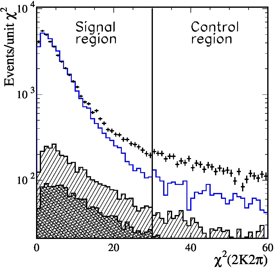 Figure 1
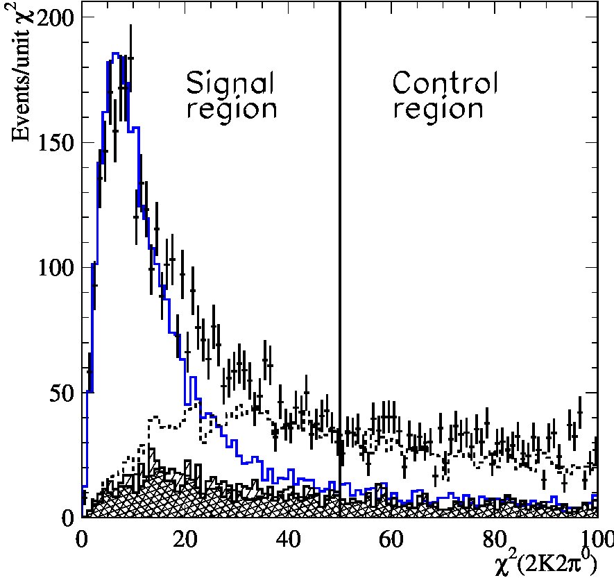 Figure 2
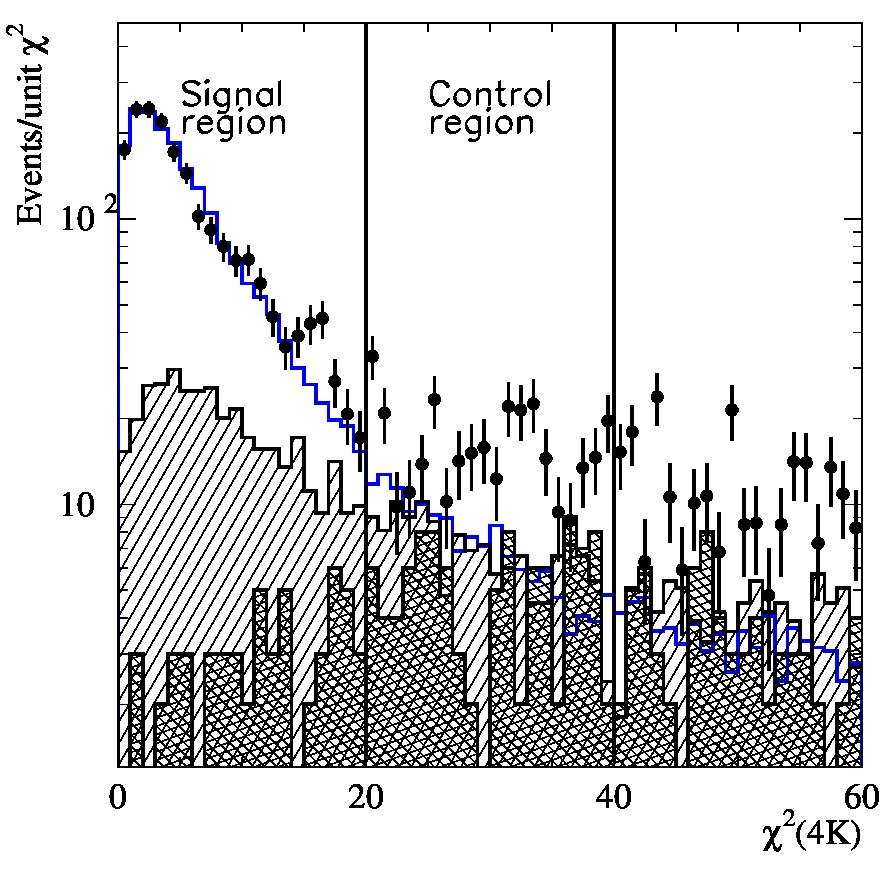 Figure 3
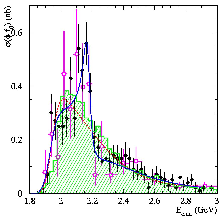 Figure 4
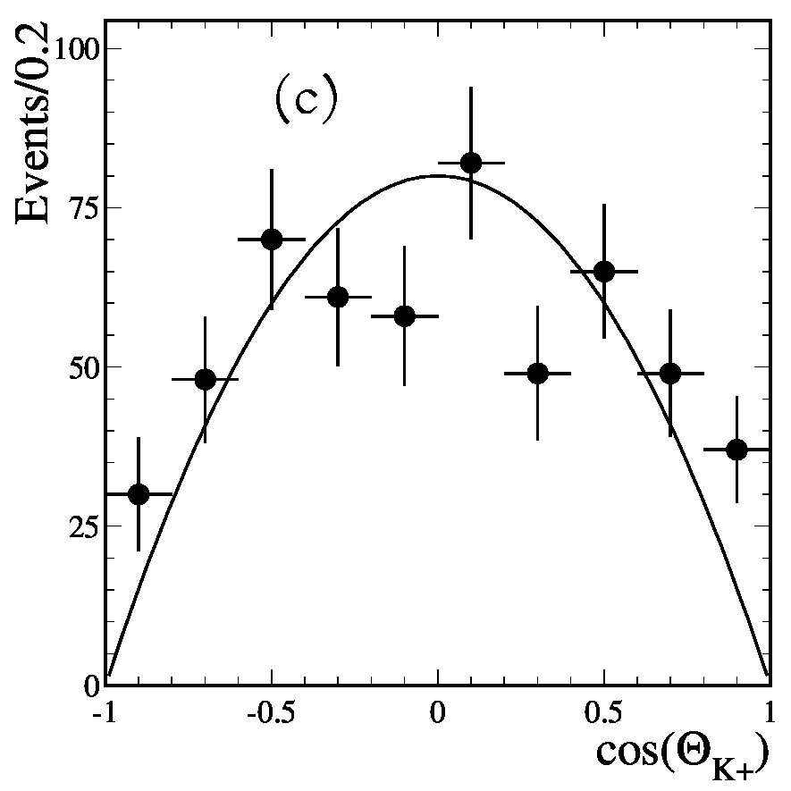 Figure 5
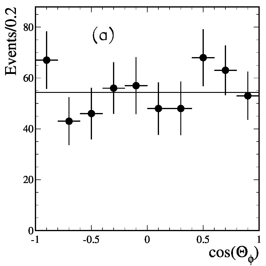 Figure 6
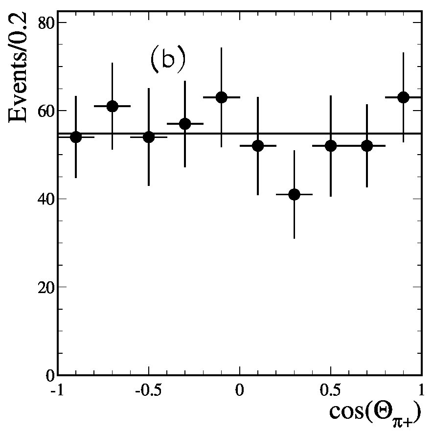 Figure 7
 Figure 8
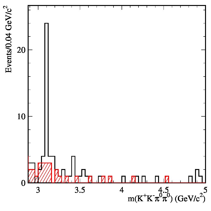 Figure 9
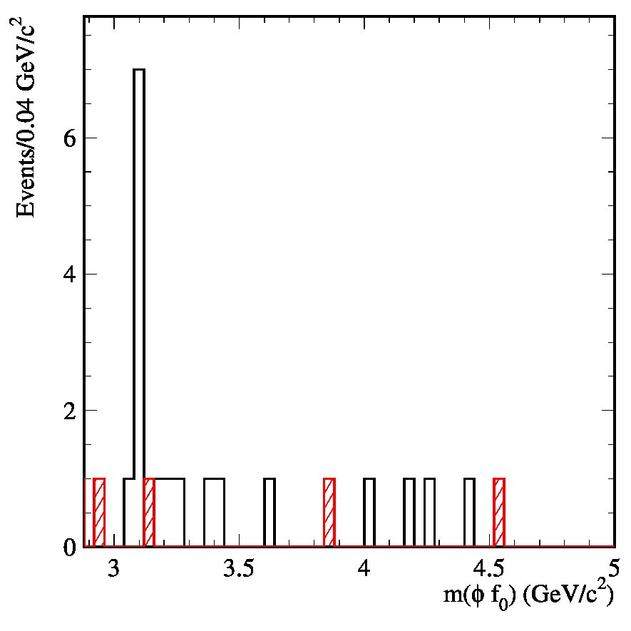 Figure 10
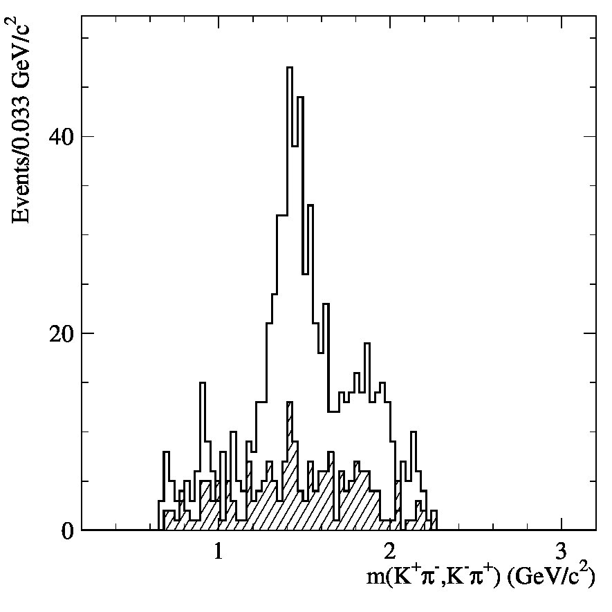 Figure 11
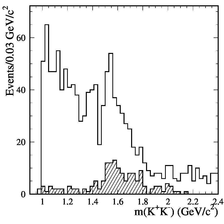 Figure 12
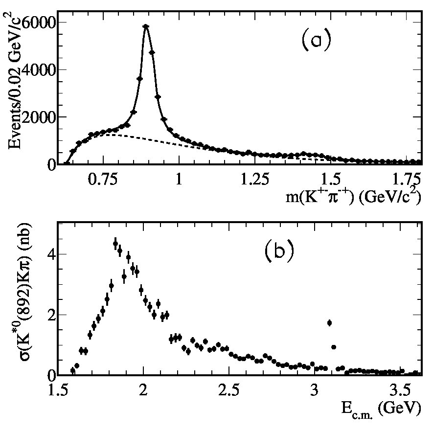 Figure 13
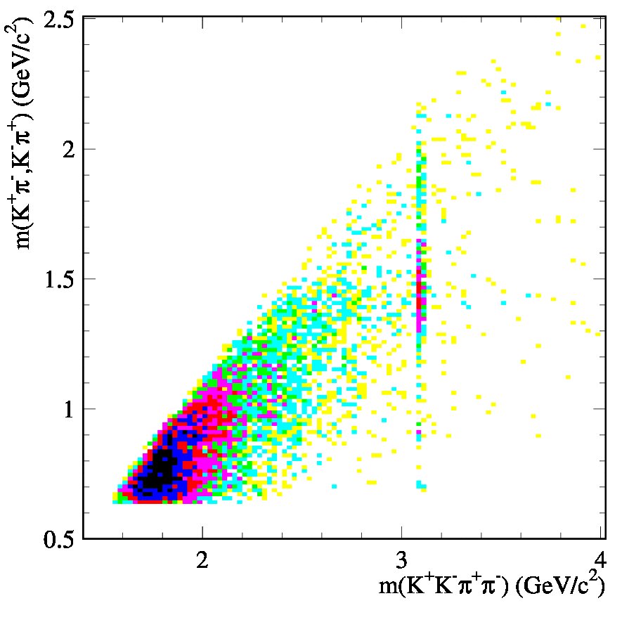 Figure 14
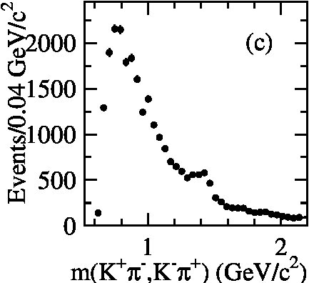 Figure 15
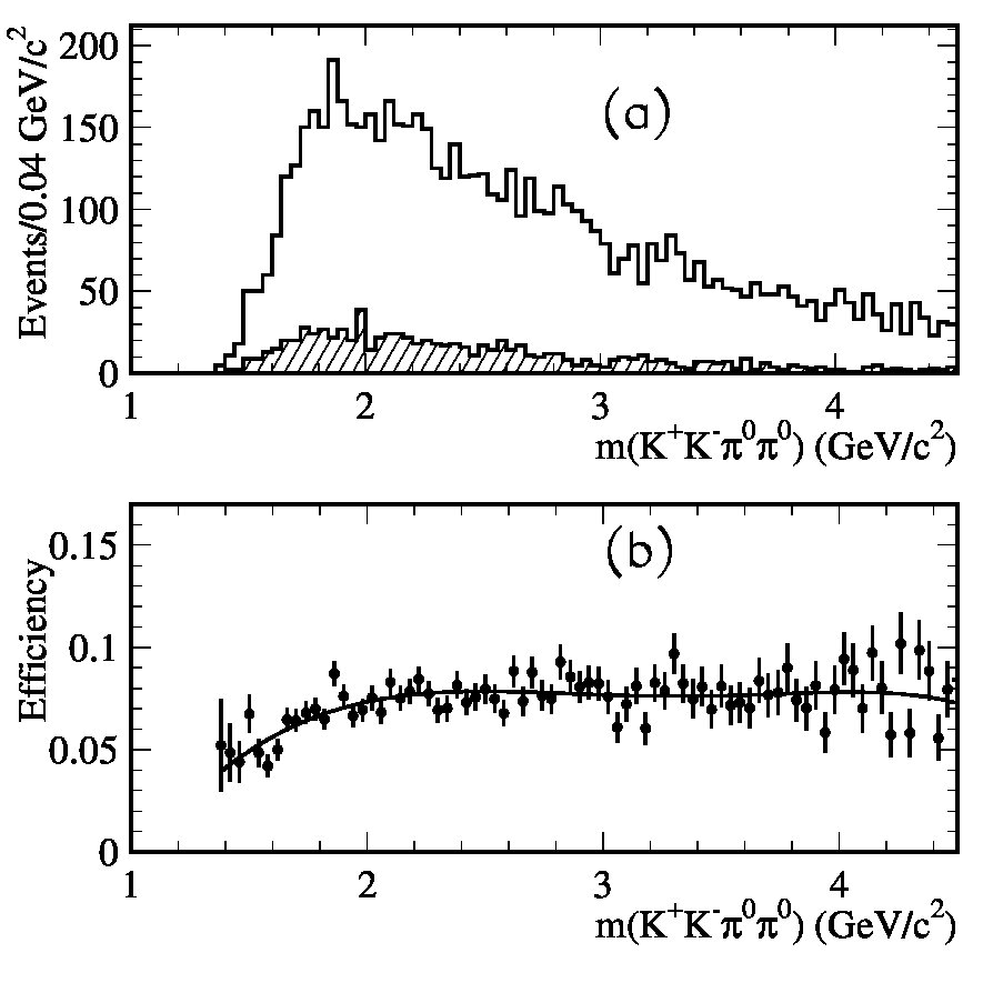 Figure 16
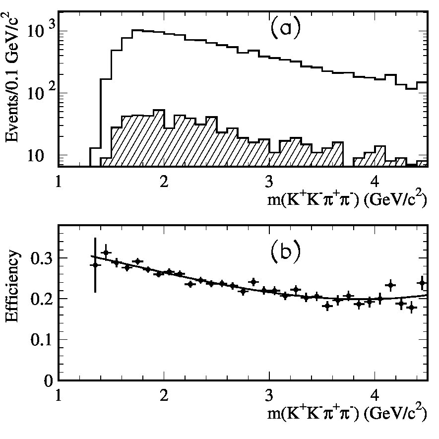 Figure 17
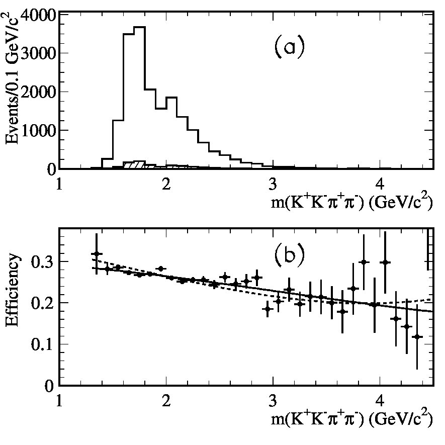 Figure 18
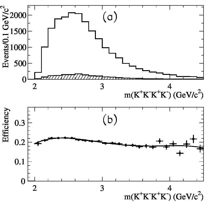 Figure 19
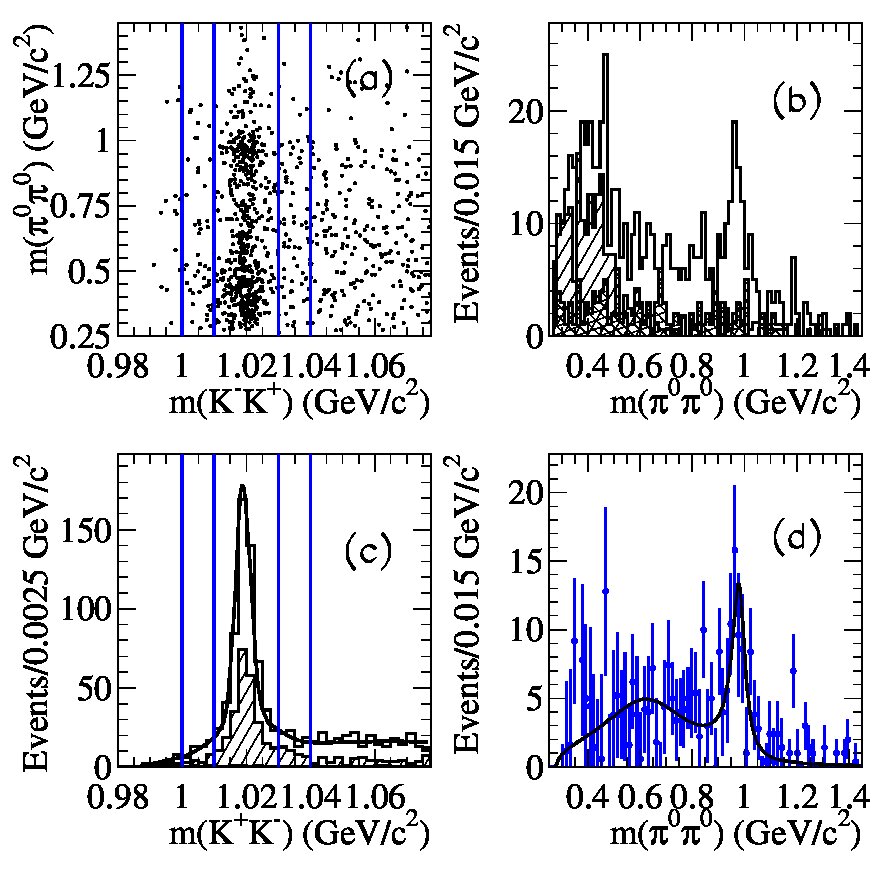 Figure 20
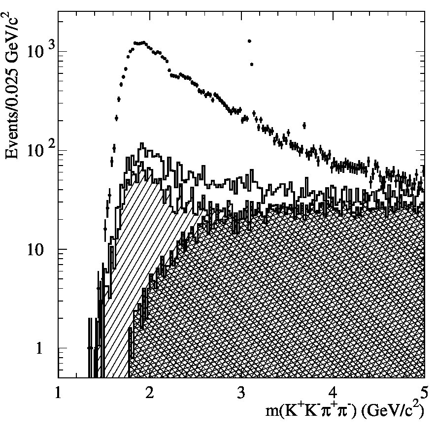 Figure 21
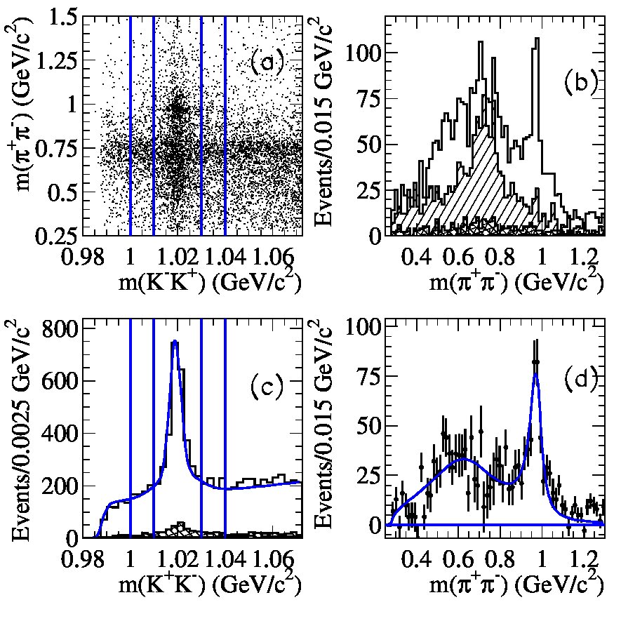 Figure 22
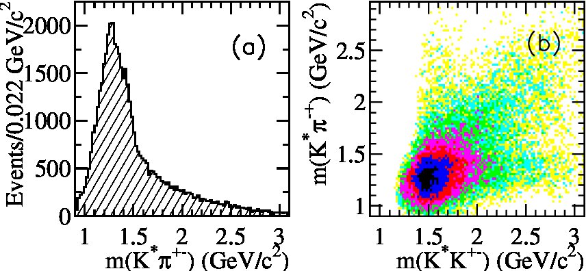 Figure 23
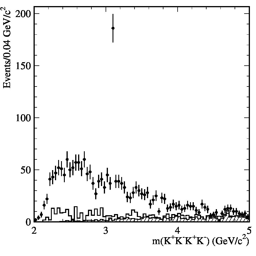 Figure 24
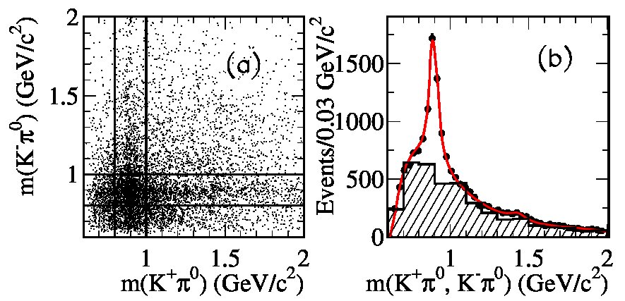 Figure 25
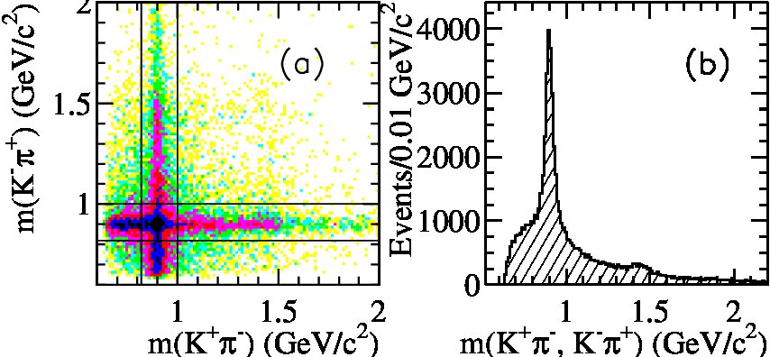 Figure 26
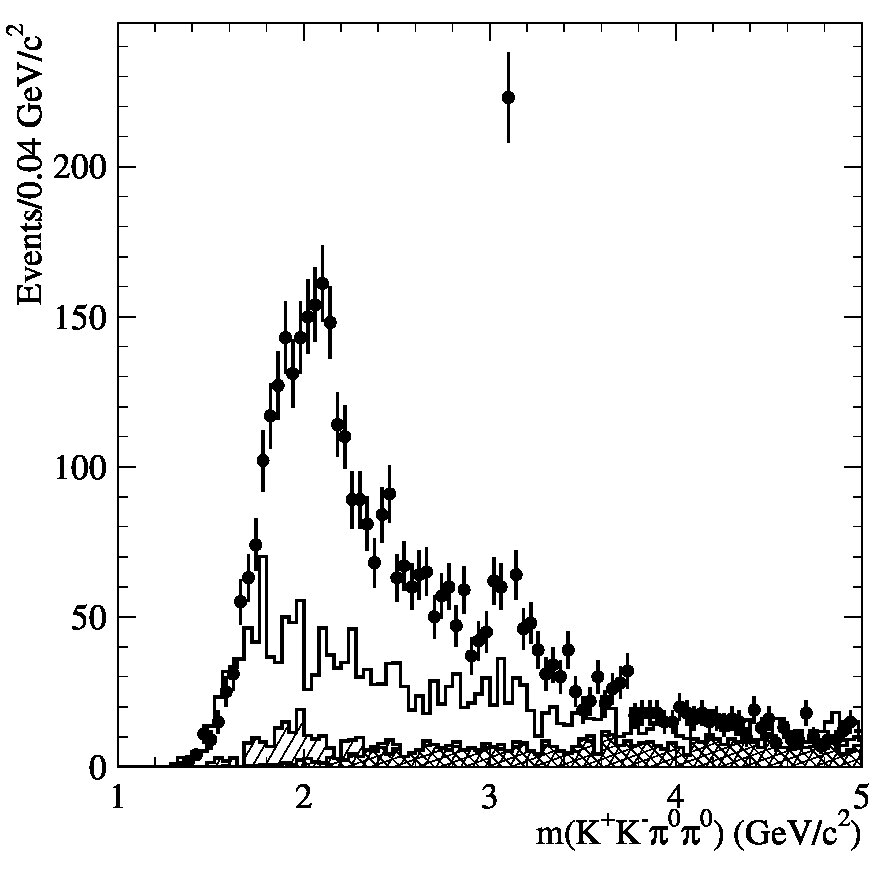 Figure 27
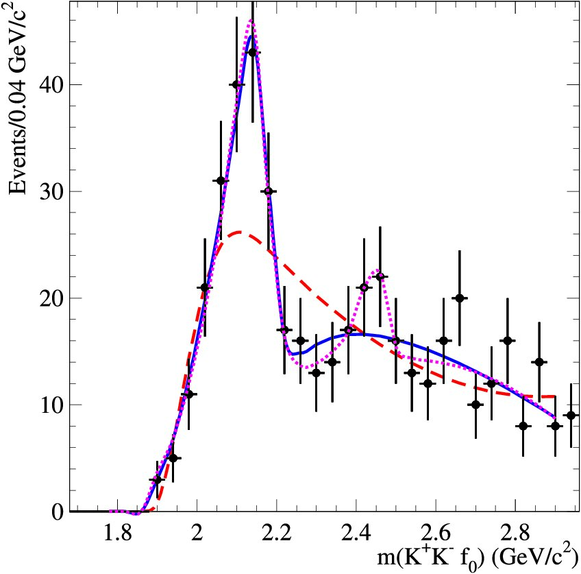 Figure 28
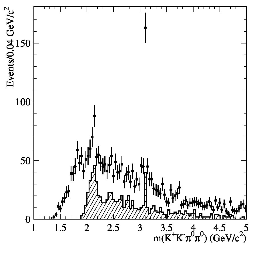 Figure 29
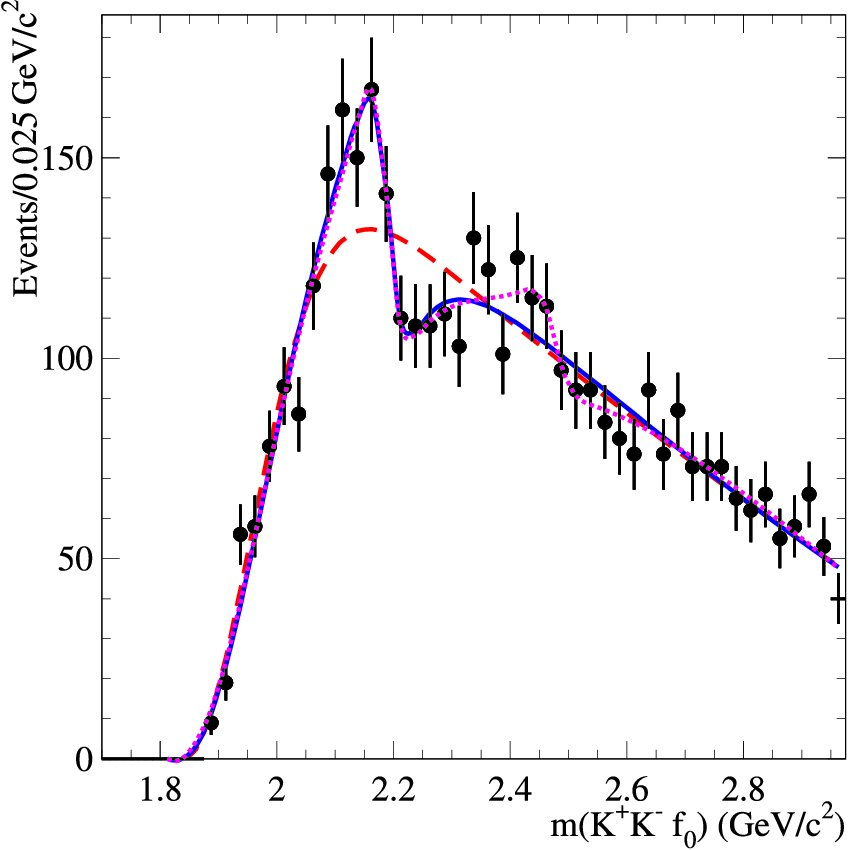 Figure 30
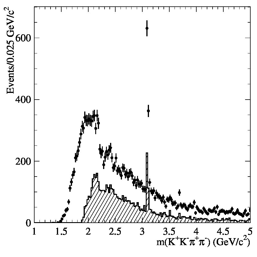 Figure 31
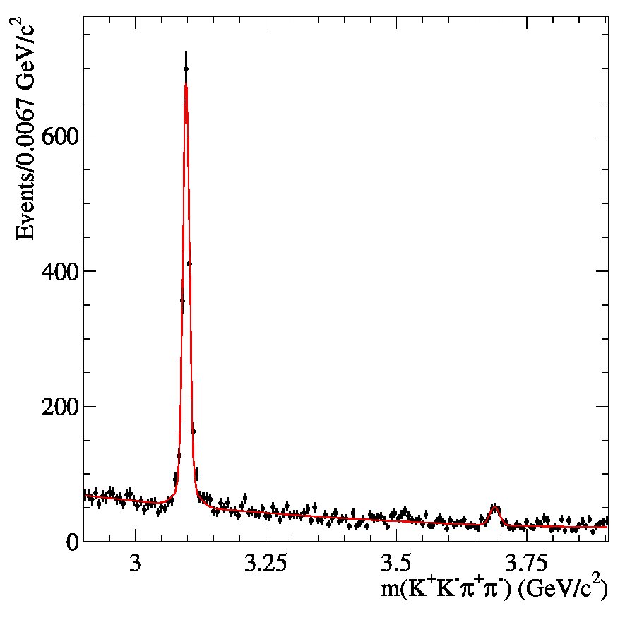 Figure 32
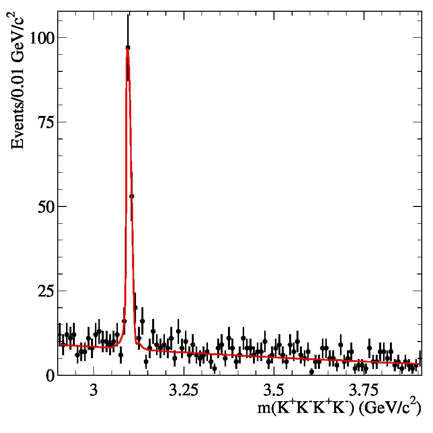 Figure 33
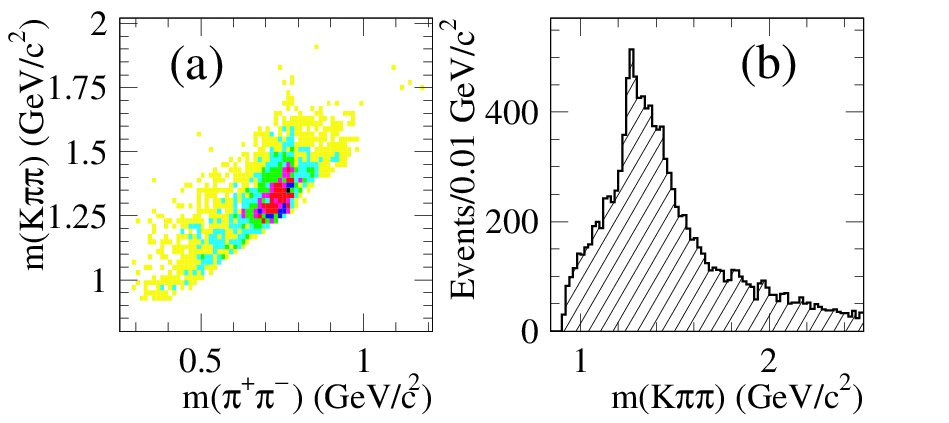 Figure 34
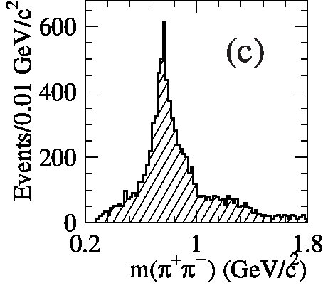 Figure 35
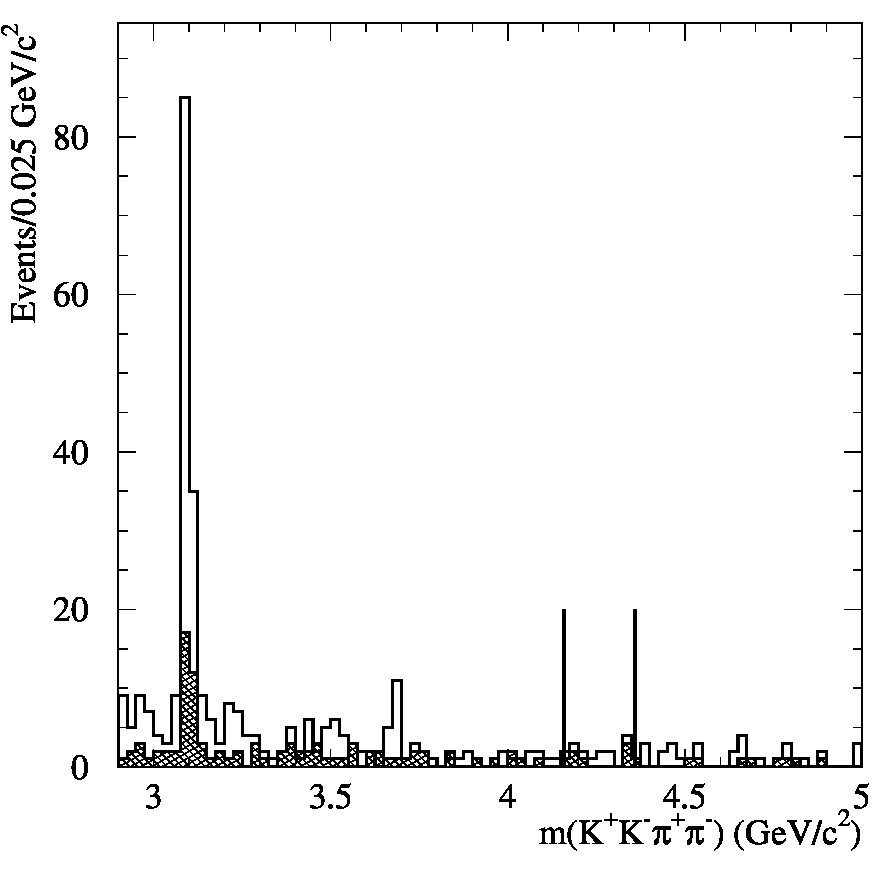 Figure 36
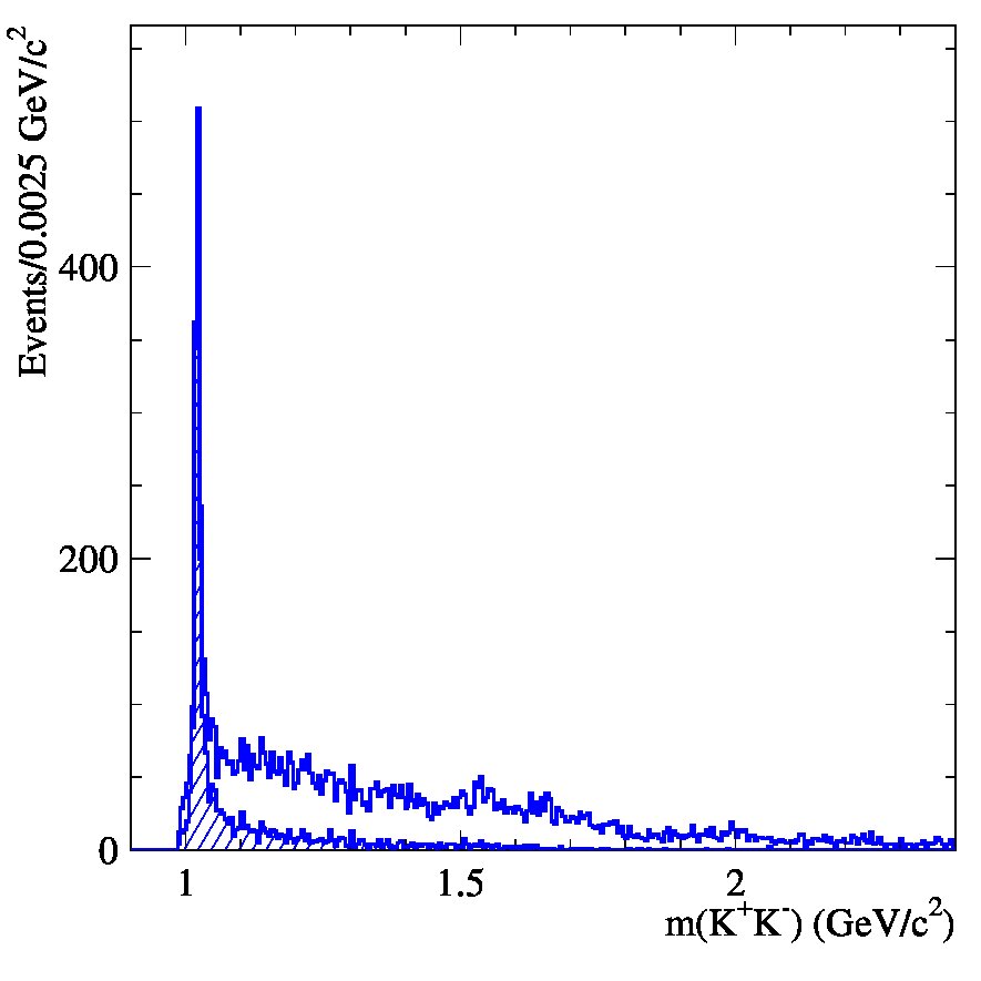 Figure 37
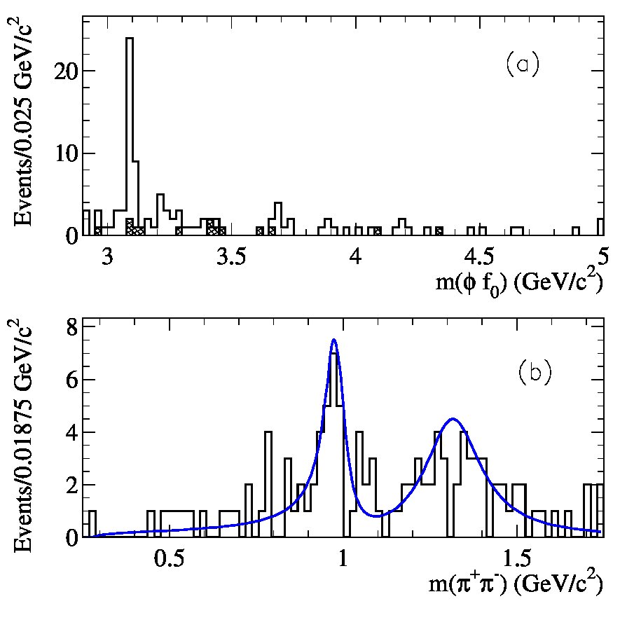 Figure 38
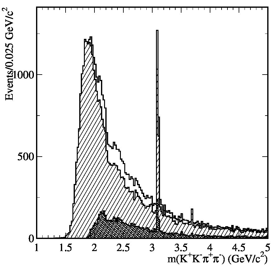 Figure 39
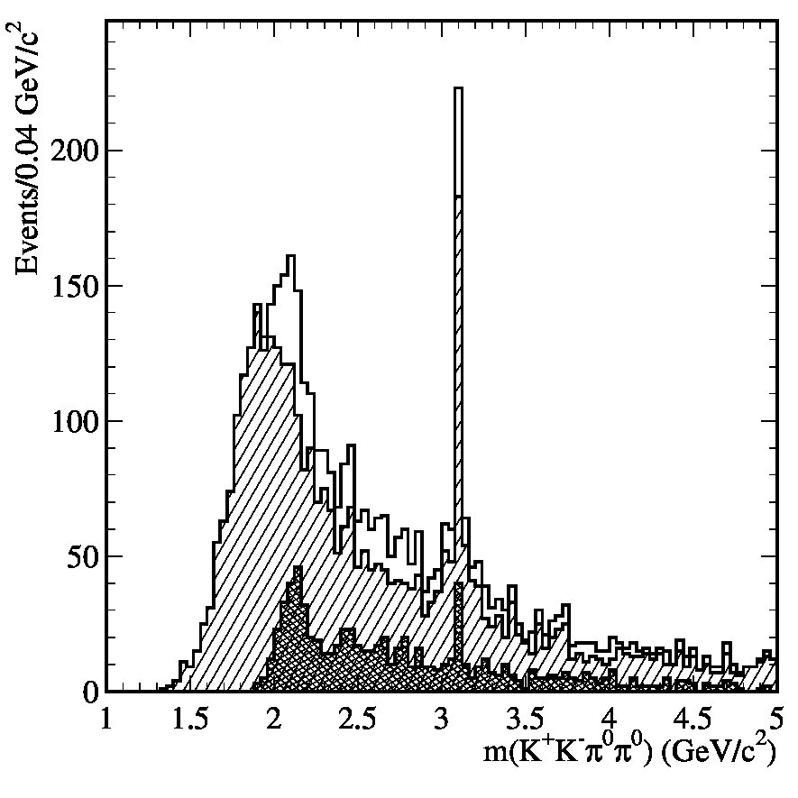 Figure 40
| (GeV) | (nb) | (GeV) | (nb) | (GeV) | (nb) | (GeV) | (nb) | (GeV) | (nb) | |||||
|---|---|---|---|---|---|---|---|---|---|---|---|---|---|---|
| 1.4125 | 0.00 | 0.02 | 2.1375 | 2.83 | 0.13 | 2.8625 | 0.50 | 0.05 | 3.5875 | 0.12 | 0.03 | 4.3125 | 0.04 | 0.02 |
| 1.4375 | 0.01 | 0.02 | 2.1625 | 2.71 | 0.12 | 2.8875 | 0.51 | 0.05 | 3.6125 | 0.13 | 0.03 | 4.3375 | 0.04 | 0.02 |
| 1.4625 | 0.00 | 0.02 | 2.1875 | 2.46 | 0.12 | 2.9125 | 0.54 | 0.05 | 3.6375 | 0.12 | 0.03 | 4.3625 | 0.03 | 0.02 |
| 1.4875 | 0.04 | 0.02 | 2.2125 | 1.84 | 0.10 | 2.9375 | 0.46 | 0.05 | 3.6625 | 0.11 | 0.03 | 4.3875 | 0.06 | 0.02 |
| 1.5125 | 0.03 | 0.02 | 2.2375 | 1.66 | 0.10 | 2.9625 | 0.45 | 0.05 | 3.6875 | 0.25 | 0.03 | 4.4125 | 0.01 | 0.02 |
| 1.5375 | 0.11 | 0.03 | 2.2625 | 1.59 | 0.09 | 2.9875 | 0.46 | 0.05 | 3.7125 | 0.07 | 0.03 | 4.4375 | 0.03 | 0.02 |
| 1.5625 | 0.15 | 0.04 | 2.2875 | 1.66 | 0.09 | 3.0125 | 0.36 | 0.04 | 3.7375 | 0.08 | 0.02 | 4.4625 | 0.06 | 0.02 |
| 1.5875 | 0.32 | 0.05 | 2.3125 | 1.50 | 0.09 | 3.0375 | 0.39 | 0.04 | 3.7625 | 0.11 | 0.03 | 4.4875 | 0.03 | 0.02 |
| 1.6125 | 0.48 | 0.06 | 2.3375 | 1.65 | 0.09 | 3.0625 | 0.31 | 0.04 | 3.7875 | 0.11 | 0.03 | 4.5125 | 0.04 | 0.02 |
| 1.6375 | 0.85 | 0.08 | 2.3625 | 1.56 | 0.09 | 3.0875 | 2.95 | 0.10 | 3.8125 | 0.10 | 0.03 | 4.5375 | 0.01 | 0.02 |
| 1.6625 | 1.42 | 0.10 | 2.3875 | 1.49 | 0.09 | 3.1125 | 1.51 | 0.08 | 3.8375 | 0.08 | 0.02 | 4.5625 | 0.02 | 0.02 |
| 1.6875 | 1.86 | 0.11 | 2.4125 | 1.46 | 0.09 | 3.1375 | 0.37 | 0.04 | 3.8625 | 0.12 | 0.03 | 4.5875 | 0.05 | 0.02 |
| 1.7125 | 2.36 | 0.13 | 2.4375 | 1.48 | 0.09 | 3.1625 | 0.35 | 0.04 | 3.8875 | 0.09 | 0.02 | 4.6125 | 0.02 | 0.02 |
| 1.7375 | 2.67 | 0.13 | 2.4625 | 1.17 | 0.08 | 3.1875 | 0.28 | 0.04 | 3.9125 | 0.09 | 0.02 | 4.6375 | 0.01 | 0.02 |
| 1.7625 | 3.51 | 0.15 | 2.4875 | 1.16 | 0.08 | 3.2125 | 0.35 | 0.04 | 3.9375 | 0.08 | 0.02 | 4.6625 | 0.04 | 0.02 |
| 1.7875 | 3.98 | 0.16 | 2.5125 | 1.21 | 0.08 | 3.2375 | 0.31 | 0.04 | 3.9625 | 0.10 | 0.02 | 4.6875 | 0.02 | 0.02 |
| 1.8125 | 4.10 | 0.16 | 2.5375 | 0.94 | 0.07 | 3.2625 | 0.30 | 0.04 | 3.9875 | 0.04 | 0.02 | 4.7125 | 0.03 | 0.02 |
| 1.8375 | 4.68 | 0.17 | 2.5625 | 0.95 | 0.07 | 3.2875 | 0.24 | 0.04 | 4.0125 | 0.06 | 0.02 | 4.7375 | 0.01 | 0.02 |
| 1.8625 | 4.49 | 0.17 | 2.5875 | 0.84 | 0.07 | 3.3125 | 0.22 | 0.04 | 4.0375 | 0.07 | 0.02 | 4.7625 | 0.02 | 0.02 |
| 1.8875 | 4.26 | 0.17 | 2.6125 | 0.85 | 0.07 | 3.3375 | 0.25 | 0.04 | 4.0625 | 0.05 | 0.02 | 4.7875 | 0.01 | 0.02 |
| 1.9125 | 4.30 | 0.16 | 2.6375 | 0.90 | 0.07 | 3.3625 | 0.16 | 0.03 | 4.0875 | 0.06 | 0.02 | 4.8125 | 0.00 | 0.02 |
| 1.9375 | 4.20 | 0.16 | 2.6625 | 0.82 | 0.06 | 3.3875 | 0.17 | 0.03 | 4.1125 | 0.06 | 0.02 | 4.8375 | 0.02 | 0.02 |
| 1.9625 | 4.13 | 0.16 | 2.6875 | 0.70 | 0.06 | 3.4125 | 0.18 | 0.03 | 4.1375 | 0.05 | 0.02 | 4.8625 | 0.00 | 0.02 |
| 1.9875 | 3.74 | 0.15 | 2.7125 | 0.86 | 0.06 | 3.4375 | 0.12 | 0.03 | 4.1625 | 0.06 | 0.02 | 4.8875 | 0.04 | 0.02 |
| 2.0125 | 3.45 | 0.15 | 2.7375 | 0.81 | 0.06 | 3.4625 | 0.17 | 0.03 | 4.1875 | 0.05 | 0.02 | 4.9125 | 0.05 | 0.02 |
| 2.0375 | 3.38 | 0.14 | 2.7625 | 0.76 | 0.06 | 3.4875 | 0.17 | 0.03 | 4.2125 | 0.05 | 0.02 | 4.9375 | 0.02 | 0.02 |
| 2.0625 | 3.17 | 0.14 | 2.7875 | 0.73 | 0.06 | 3.5125 | 0.21 | 0.03 | 4.2375 | 0.08 | 0.02 | 4.9625 | 0.00 | 0.02 |
| 2.0875 | 3.23 | 0.14 | 2.8125 | 0.64 | 0.05 | 3.5375 | 0.14 | 0.03 | 4.2625 | 0.04 | 0.02 | 4.9875 | 0.04 | 0.02 |
| 2.1125 | 3.15 | 0.14 | 2.8375 | 0.56 | 0.05 | 3.5625 | 0.16 | 0.03 | 4.2875 | 0.08 | 0.02 | |||
| Source | Correction | Uncertainty |
| Rad. Corrections | – | |
| Backgrounds | – | , |
| , | ||
| Model Dependence | – | |
| Distn. | ||
| Tracking Efficiency | ||
| Kaon ID Efficiency | ||
| ISR Luminosity | – | |
| Total | , | |
| , |
| (GeV) | (nb) | (GeV) | (nb) | (GeV) | (nb) | (GeV) | (nb) |
|---|---|---|---|---|---|---|---|
| 1.5875 | 0.16 0.11 | 2.0875 | 2.36 0.16 | 2.5875 | 0.54 0.07 | 3.0875 | 1.73 0.10 |
| 1.6125 | 0.31 0.08 | 2.1125 | 1.92 0.16 | 2.6125 | 0.63 0.06 | 3.1125 | 0.92 0.07 |
| 1.6375 | 0.81 0.13 | 2.1375 | 1.99 0.14 | 2.6375 | 0.57 0.06 | 3.1375 | 0.21 0.04 |
| 1.6625 | 0.79 0.12 | 2.1625 | 1.19 0.15 | 2.6625 | 0.46 0.06 | 3.1625 | 0.24 0.04 |
| 1.6875 | 1.33 0.15 | 2.1875 | 1.24 0.14 | 2.6875 | 0.46 0.06 | 3.1875 | 0.08 0.03 |
| 1.7125 | 1.63 0.15 | 2.2125 | 1.25 0.11 | 2.7125 | 0.64 0.06 | 3.2125 | 0.15 0.03 |
| 1.7375 | 1.87 0.14 | 2.2375 | 0.90 0.10 | 2.7375 | 0.56 0.06 | 3.2375 | 0.14 0.04 |
| 1.7625 | 2.12 0.17 | 2.2625 | 0.79 0.11 | 2.7625 | 0.46 0.06 | 3.2625 | 0.16 0.03 |
| 1.7875 | 2.51 0.20 | 2.2875 | 1.15 0.10 | 2.7875 | 0.36 0.06 | 3.2875 | 0.13 0.03 |
| 1.8125 | 2.96 0.21 | 2.3125 | 0.99 0.09 | 2.8125 | 0.31 0.05 | 3.3125 | 0.12 0.03 |
| 1.8375 | 4.35 0.20 | 2.3375 | 0.91 0.11 | 2.8375 | 0.35 0.05 | 3.3375 | 0.14 0.03 |
| 1.8625 | 4.11 0.20 | 2.3625 | 1.11 0.09 | 2.8625 | 0.27 0.04 | 3.3625 | 0.12 0.06 |
| 1.8875 | 3.26 0.23 | 2.3875 | 0.83 0.09 | 2.8875 | 0.27 0.05 | 3.3875 | 0.09 0.03 |
| 1.9125 | 3.90 0.20 | 2.4125 | 0.87 0.09 | 2.9125 | 0.34 0.05 | 3.4125 | 0.10 0.03 |
| 1.9375 | 3.53 0.20 | 2.4375 | 1.00 0.09 | 2.9375 | 0.29 0.04 | 3.4375 | 0.11 0.03 |
| 1.9625 | 3.42 0.21 | 2.4625 | 0.86 0.08 | 2.9625 | 0.25 0.04 | 3.4625 | 0.10 0.05 |
| 1.9875 | 2.81 0.18 | 2.4875 | 0.88 0.09 | 2.9875 | 0.38 0.05 | 3.4875 | 0.08 0.03 |
| 2.0125 | 2.47 0.17 | 2.5125 | 0.69 0.07 | 3.0125 | 0.21 0.04 | ||
| 2.0375 | 2.26 0.16 | 2.5375 | 0.62 0.07 | 3.0375 | 0.24 0.04 | ||
| 2.0625 | 2.00 0.16 | 2.5625 | 0.55 0.07 | 3.0625 | 0.22 0.04 |
| (GeV) | (nb) | (GeV) | (nb) | (GeV) | (nb) | (GeV) | (nb) |
|---|---|---|---|---|---|---|---|
| 1.4875 | 0.01 0.02 | 1.8375 | 0.39 0.10 | 2.1875 | 0.32 0.06 | 2.5375 | 0.09 0.03 |
| 1.5125 | 0.03 0.03 | 1.8625 | 0.44 0.10 | 2.2125 | 0.22 0.05 | 2.5625 | 0.03 0.02 |
| 1.5375 | 0.09 0.04 | 1.8875 | 0.23 0.08 | 2.2375 | 0.15 0.04 | 2.5875 | 0.06 0.02 |
| 1.5625 | 0.13 0.04 | 1.9125 | 0.34 0.09 | 2.2625 | 0.10 0.03 | 2.6125 | 0.07 0.02 |
| 1.5875 | 0.21 0.06 | 1.9375 | 0.37 0.08 | 2.2875 | 0.11 0.04 | 2.6375 | 0.08 0.03 |
| 1.6125 | 0.23 0.06 | 1.9625 | 0.31 0.08 | 2.3125 | 0.08 0.03 | 2.6625 | 0.06 0.02 |
| 1.6375 | 0.54 0.08 | 1.9875 | 0.36 0.07 | 2.3375 | 0.13 0.03 | 2.6875 | 0.04 0.02 |
| 1.6625 | 0.61 0.09 | 2.0125 | 0.38 0.07 | 2.3625 | 0.10 0.04 | 2.7125 | 0.08 0.03 |
| 1.6875 | 0.64 0.10 | 2.0375 | 0.29 0.07 | 2.3875 | 0.13 0.04 | 2.7375 | 0.06 0.02 |
| 1.7125 | 0.38 0.09 | 2.0625 | 0.42 0.07 | 2.4125 | 0.12 0.04 | 2.7625 | 0.07 0.02 |
| 1.7375 | 0.64 0.10 | 2.0875 | 0.30 0.06 | 2.4375 | 0.15 0.04 | 2.7875 | 0.02 0.02 |
| 1.7625 | 0.55 0.11 | 2.1125 | 0.49 0.07 | 2.4625 | 0.06 0.03 | 2.8125 | 0.06 0.02 |
| 1.7875 | 0.55 0.11 | 2.1375 | 0.30 0.06 | 2.4875 | 0.09 0.03 | 2.8375 | 0.04 0.02 |
| 1.8125 | 0.31 0.09 | 2.1625 | 0.49 0.07 | 2.5125 | 0.09 0.03 | 2.8625 | 0.03 0.01 |
| (GeV) | (nb) | (GeV) | (nb) | (GeV) | (nb) | (GeV) | (nb) |
|---|---|---|---|---|---|---|---|
| 1.8875 | 0.02 0.02 | 2.1625 | 0.56 0.08 | 2.4375 | 0.13 0.04 | 2.7125 | 0.05 0.02 |
| 1.9125 | 0.07 0.04 | 2.1875 | 0.38 0.07 | 2.4625 | 0.09 0.04 | 2.7375 | 0.02 0.01 |
| 1.9375 | 0.30 0.07 | 2.2125 | 0.21 0.06 | 2.4875 | 0.08 0.03 | 2.7625 | 0.06 0.02 |
| 1.9625 | 0.27 0.07 | 2.2375 | 0.17 0.05 | 2.5125 | 0.09 0.03 | 2.7875 | 0.03 0.02 |
| 1.9875 | 0.25 0.07 | 2.2625 | 0.12 0.04 | 2.5375 | 0.07 0.03 | 2.8125 | 0.04 0.02 |
| 2.0125 | 0.25 0.07 | 2.2875 | 0.13 0.05 | 2.5625 | 0.02 0.02 | 2.8375 | 0.05 0.02 |
| 2.0375 | 0.28 0.07 | 2.3125 | 0.12 0.04 | 2.5875 | 0.06 0.03 | 2.8625 | 0.02 0.02 |
| 2.0625 | 0.43 0.08 | 2.3375 | 0.14 0.04 | 2.6125 | 0.07 0.03 | 2.8875 | 0.01 0.01 |
| 2.0875 | 0.28 0.07 | 2.3625 | 0.13 0.05 | 2.6375 | 0.06 0.03 | 2.9125 | 0.02 0.01 |
| 2.1125 | 0.54 0.09 | 2.3875 | 0.13 0.04 | 2.6625 | 0.05 0.03 | 2.9375 | 0.00 0.00 |
| 2.1375 | 0.46 0.08 | 2.4125 | 0.14 0.05 | 2.6875 | 0.03 0.02 | 2.9625 | 0.02 0.01 |
| (GeV) | (nb) | (GeV) | (nb) | (GeV) | (nb) | (GeV) | (nb) |
|---|---|---|---|---|---|---|---|
| 1.4200 | 0.00 0.05 | 2.3400 | 0.35 0.06 | 3.2600 | 0.13 0.03 | 4.1800 | 0.02 0.01 |
| 1.4600 | 0.12 0.07 | 2.3800 | 0.29 0.06 | 3.3000 | 0.09 0.03 | 4.2200 | 0.03 0.01 |
| 1.5000 | 0.00 0.07 | 2.4200 | 0.38 0.06 | 3.3400 | 0.09 0.03 | 4.2600 | 0.03 0.01 |
| 1.5400 | 0.01 0.08 | 2.4600 | 0.38 0.06 | 3.3800 | 0.08 0.02 | 4.3000 | 0.03 0.01 |
| 1.5800 | 0.03 0.09 | 2.5000 | 0.22 0.05 | 3.4200 | 0.11 0.03 | 4.3400 | 0.03 0.01 |
| 1.6200 | 0.09 0.09 | 2.5400 | 0.25 0.05 | 3.4600 | 0.06 0.02 | 4.3800 | 0.01 0.01 |
| 1.6600 | 0.31 0.11 | 2.5800 | 0.25 0.05 | 3.5000 | 0.04 0.02 | 4.4200 | 0.05 0.01 |
| 1.7000 | 0.35 0.11 | 2.6200 | 0.25 0.05 | 3.5400 | 0.06 0.02 | 4.4600 | 0.03 0.01 |
| 1.7400 | 0.49 0.11 | 2.6600 | 0.28 0.05 | 3.5800 | 0.07 0.02 | 4.5000 | 0.04 0.01 |
| 1.7800 | 0.51 0.12 | 2.7000 | 0.16 0.04 | 3.6200 | 0.04 0.02 | 4.5400 | 0.00 0.01 |
| 1.8200 | 0.84 0.12 | 2.7400 | 0.22 0.04 | 3.6600 | 0.06 0.02 | 4.5800 | 0.02 0.01 |
| 1.8600 | 0.94 0.11 | 2.7800 | 0.21 0.04 | 3.7000 | 0.08 0.02 | 4.6200 | 0.02 0.01 |
| 1.9000 | 0.95 0.12 | 2.8200 | 0.13 0.04 | 3.7400 | 0.09 0.02 | 4.6600 | 0.02 0.01 |
| 1.9400 | 0.80 0.11 | 2.8600 | 0.21 0.04 | 3.7800 | 0.02 0.02 | 4.7000 | 0.04 0.01 |
| 1.9800 | 0.87 0.11 | 2.9000 | 0.11 0.03 | 3.8200 | 0.05 0.01 | 4.7400 | 0.02 0.01 |
| 2.0200 | 1.00 0.10 | 2.9400 | 0.12 0.04 | 3.8600 | 0.04 0.01 | 4.7800 | 0.01 0.01 |
| 2.0600 | 0.96 0.10 | 2.9800 | 0.12 0.04 | 3.9000 | 0.03 0.02 | 4.8200 | 0.01 0.01 |
| 2.1000 | 0.90 0.10 | 3.0200 | 0.21 0.04 | 3.9400 | 0.02 0.01 | 4.8600 | 0.01 0.01 |
| 2.1400 | 0.82 0.10 | 3.0600 | 0.16 0.04 | 3.9800 | 0.03 0.01 | 4.9000 | 0.03 0.01 |
| 2.1800 | 0.58 0.08 | 3.1000 | 0.92 0.07 | 4.0200 | 0.05 0.01 | 4.9400 | 0.04 0.02 |
| 2.2200 | 0.56 0.08 | 3.1400 | 0.19 0.04 | 4.0600 | 0.04 0.01 | 4.9800 | 0.04 0.02 |
| 2.2600 | 0.37 0.07 | 3.1800 | 0.12 0.03 | 4.1000 | 0.03 0.01 | ||
| 2.3000 | 0.43 0.07 | 3.2200 | 0.14 0.03 | 4.1400 | 0.03 0.01 |
| Source | Correction | Uncertainty | |
|---|---|---|---|
| Rad. Corrections | – | ||
| Backgrounds | – | , | |
| , | |||
| Model Dependence | – | ||
| Distn. | 0% | ||
| Tracking Efficiency | |||
| Kaon ID Efficiency | |||
| Efficiency | |||
| ISR Luminosity | – | ||
| Total | , | ||
| , | |||
| (GeV) | (nb) | (GeV) | (nb) | (GeV) | (nb) |
|---|---|---|---|---|---|
| 1.88-1.92 | 2.12-2.16 | 2.44-2.52 | |||
| 1.92-1.96 | 2.16-2.20 | 2.52-2.68 | |||
| 1.96-2.00 | 2.20-2.24 | 2.68-2.84 | |||
| 2.00-2.04 | 2.24-2.28 | 2.84-3.00 | |||
| 2.04-2.08 | 2.28-2.36 | 3.00-3.16 | |||
| 2.08-2.12 | 2.36-2.44 | 3.16-3.32 |
| (GeV) | (nb) | (GeV) | (nb) | (GeV) | (nb) | (GeV) | (nb) |
|---|---|---|---|---|---|---|---|
| 2.02 | 0.006 0.004 | 2.66 | 0.075 0.015 | 3.30 | 0.025 0.009 | 3.94 | 0.012 0.006 |
| 2.06 | 0.011 0.006 | 2.70 | 0.102 0.015 | 3.34 | 0.025 0.009 | 3.98 | 0.012 0.006 |
| 2.10 | 0.019 0.007 | 2.74 | 0.069 0.014 | 3.38 | 0.024 0.010 | 4.02 | 0.010 0.006 |
| 2.14 | 0.034 0.011 | 2.78 | 0.063 0.014 | 3.42 | 0.034 0.010 | 4.06 | 0.009 0.005 |
| 2.18 | 0.040 0.013 | 2.82 | 0.051 0.012 | 3.46 | 0.036 0.009 | 4.10 | 0.006 0.005 |
| 2.22 | 0.087 0.016 | 2.86 | 0.024 0.011 | 3.50 | 0.032 0.009 | 4.14 | 0.008 0.006 |
| 2.26 | 0.064 0.018 | 2.90 | 0.054 0.012 | 3.54 | 0.025 0.009 | 4.18 | 0.011 0.005 |
| 2.30 | 0.082 0.017 | 2.94 | 0.045 0.013 | 3.58 | 0.031 0.009 | 4.22 | 0.011 0.005 |
| 2.34 | 0.079 0.018 | 2.98 | 0.045 0.011 | 3.62 | 0.014 0.007 | 4.26 | 0.012 0.005 |
| 2.38 | 0.084 0.017 | 3.02 | 0.063 0.013 | 3.66 | 0.019 0.008 | 4.30 | 0.004 0.005 |
| 2.42 | 0.070 0.016 | 3.06 | 0.049 0.012 | 3.70 | 0.028 0.008 | 4.34 | 0.003 0.006 |
| 2.46 | 0.092 0.018 | 3.10 | 0.287 0.024 | 3.74 | 0.008 0.005 | 4.38 | 0.013 0.005 |
| 2.50 | 0.082 0.015 | 3.14 | 0.050 0.012 | 3.78 | 0.026 0.007 | 4.42 | 0.012 0.005 |
| 2.54 | 0.091 0.015 | 3.18 | 0.054 0.011 | 3.82 | 0.020 0.007 | 4.46 | 0.006 -0.004 |
| 2.58 | 0.077 0.017 | 3.22 | 0.049 0.011 | 3.86 | 0.007 0.006 | 4.50 | -0.001 -0.004 |
| 2.62 | 0.095 0.015 | 3.26 | 0.045 0.010 | 3.90 | 0.012 0.006 | 4.54 | 0.000 0.004 |
| Source | Correction | Uncertainty | |
|---|---|---|---|
| Rad. Corrections | – | ||
| Backgrounds | – | ||
| Model Dependence | – | ||
| Distribution | |||
| Tracking Efficiency | |||
| Kaon ID Efficiency | |||
| ISR Luminosity | – | ||
| Total | |||
| Fit | All fixed | Only fixed | All free | ||||||
|---|---|---|---|---|---|---|---|---|---|
| 1.19 | 0.03 | 1.23 | 0.03 | 1.09 | 0.01 | ||||
| 0.218* | 0.218* | 0.174 | 0.012 | ||||||
| 1.68* | 1.51 | 0.15 | 1.49 | 0.12 | |||||
| 0.81* | 0.66 | 0.14 | 0.63 | 0.11 | |||||
| /n.d.f. | 86.4/54 | 85.3/52 | 80.5/51 | ||||||
| P() | 0.0035 | 0.0025 | 0.0053 | ||||||
| No Resonance | One Resonance | Two Resonances | ||||
|---|---|---|---|---|---|---|
| Fit | ||||||
| 7204775 | 991202 | 8466334 | 722112 | 6502476 | 11789 | |
| 0.1810.012 | 0.1340.017 | 0.2240.024 | 0.1970.048 | 0.2010.035 | 0.1430.053 | |
| 0.750.21 | 1.470.38 | 0.890.17 | 0.360.10 | 0.440.15 | 5.802.36 | |
| 0.090.17 | 0.750.35 | 0.170.08 | 0.280.14 | 0.150.12 | 5.261.75 | |
| 0.75* | 0.50* | 0.75* | 0.50* | 0.75* | 0.50* | |
| 0* | 0* | 11695 | 14936 | 16370 | 19244 | |
| () | – | – | 2.1920.014 | 2.1690.020 | 2.1870.013 | 2.1540.029 |
| () | – | – | 0.0710.021 | 0.1020.027 | 0.0660.018 | 0.1100.022 |
| (rad) | – | – | 0.600.41 | 1.020.19 | 1.100.14 | 1.040.23 |
| 0* | 0* | 0* | 0* | 1616 | 65 | |
| () | – | – | – | – | 2.470.07 | 2.450.04 |
| () | – | – | – | – | 0.0770.065 | 0.0620.102 |
| (rad) | – | – | – | – | 0.281.06 | 1.411.29 |
| /n.d.f. | 62.8/41 | 38.1/21 | 35.6/37 | 13.0/17 | 31.4/34 | 9.7/13 |
| P() | 0.016 | 0.012 | 0.54 | 0.74 | 0.60 | 0.72 |
| Measured | Measured | or Branching Fraction (10-3) | ||||||||||
|---|---|---|---|---|---|---|---|---|---|---|---|---|
| Quantity | Value () | Calculated, this work | PDG2006 | |||||||||
| 36. | 3 | 1.3 | 2.1 | 6. | 72 | 0.24 | 0.40 | 6. | 2 | 0.7 | ||
| 13. | 6 | 1.1 | 1.3 | 2. | 52 | 0.20 | 0.25 | no entry | ||||
| 4. | 11 | 0.39 | 0.30 | 0. | 76 | 0.07 | 0.06 | 0. | 78 | 0.14 | ||
| 7. | 3 | 0.5 | 0.6 | 2. | 7 | 0.2 | 0.2 | 6. | 7 | 2.6 | ||
| 0. | 57 | 0.18 | 0.05 | 0. | 11 | 0.04 | 0.01 | 0. | 5 at 90% C.L. | |||
| 2. | 5 | 0.3 | 0.2 | – | no entry | |||||||
| 2. | 61 | 0.30 | 0.18 | 0. | 98 | 0.11 | 0.07 | 0. | 94 | 0.15 | ||
| 1. | 54 | 0.40 | 0.16 | 0. | 58 | 0.15 | 0.06 | no entry | ||||
| 0. | 50 | 0.11 | 0.04 | 0. | 28 | 0.07 | 0.02 | 0. | 32 | 0.09 (s=1.9) | ||
| 0. | 47 | 0.19 | 0.05 | 0. | 54 | 0.21 | 0.05 | 0. | 32 | 0.09 (s=1.9) | ||
| 1. | 12 | 0.18 | 0.09 | 0. | 50 | 0.08 | 0.04 | 0. | 37 at 90% C.L. | |||
| 2. | 56 | 0.42 | 0.16 | 1. | 2 | 0.2 | 0.08 | 0. | 72 | 0.05 | ||
| 0. | 28 | 0.11 | 0.02 | 0. | 27 | 0.11 | 0.02 | 0. | 113 | 0.029 | ||
| 0. | 17 | 0.08 | 0.02 | 0. | 26 | 0.12 | 0.03 | 0. | 090 | 0.033 | ||
Peer Reviews
No public reviews on file for this paper yet. If you reviewed it on a platform where reviews are public (OpenReview, ICLR, NeurIPS, ICML), you can paste yours below so the community can read it here.
Videos
No videos yet. Explain this paper in a talk, walkthrough, or lecture? Add one.
BABAR-PUB-07/021
SLAC-PUB-12435
Phys. Rev. D76, 012008 (2007)
††thanks: Deceased
The BABAR Collaboration
The , and
Cross Sections Measured with Initial-State Radiation
B. Aubert
M. Bona
D. Boutigny
Y. Karyotakis
J. P. Lees
V. Poireau
X. Prudent
V. Tisserand
A. Zghiche
Laboratoire de Physique des Particules, IN2P3/CNRS et Université de Savoie, F-74941 Annecy-Le-Vieux, France
J. Garra Tico
E. Grauges
Universitat de Barcelona, Facultat de Fisica, Departament ECM, E-08028 Barcelona, Spain
L. Lopez
A. Palano
Università di Bari, Dipartimento di Fisica and INFN, I-70126 Bari, Italy
G. Eigen
B. Stugu
L. Sun
University of Bergen, Institute of Physics, N-5007 Bergen, Norway
G. S. Abrams
M. Battaglia
D. N. Brown
J. Button-Shafer
R. N. Cahn
Y. Groysman
R. G. Jacobsen
J. A. Kadyk
L. T. Kerth
Yu. G. Kolomensky
G. Kukartsev
D. Lopes Pegna
G. Lynch
L. M. Mir
T. J. Orimoto
M. T. Ronan
K. Tackmann
W. A. Wenzel
Lawrence Berkeley National Laboratory and University of California, Berkeley, California 94720, USA
P. del Amo Sanchez
C. M. Hawkes
A. T. Watson
University of Birmingham, Birmingham, B15 2TT, United Kingdom
T. Held
H. Koch
B. Lewandowski
M. Pelizaeus
T. Schroeder
M. Steinke
Ruhr Universität Bochum, Institut für Experimentalphysik 1, D-44780 Bochum, Germany
D. Walker
University of Bristol, Bristol BS8 1TL, United Kingdom
D. J. Asgeirsson
T. Cuhadar-Donszelmann
B. G. Fulsom
C. Hearty
N. S. Knecht
T. S. Mattison
J. A. McKenna
University of British Columbia, Vancouver, British Columbia, Canada V6T 1Z1
M. Barrett
A. Khan
M. Saleem
L. Teodorescu
Brunel University, Uxbridge, Middlesex UB8 3PH, United Kingdom
V. E. Blinov
A. D. Bukin
V. P. Druzhinin
V. B. Golubev
A. P. Onuchin
S. I. Serednyakov
Yu. I. Skovpen
E. P. Solodov
K. Yu Todyshev
Budker Institute of Nuclear Physics, Novosibirsk 630090, Russia
M. Bondioli
S. Curry
I. Eschrich
D. Kirkby
A. J. Lankford
P. Lund
M. Mandelkern
E. C. Martin
D. P. Stoker
University of California at Irvine, Irvine, California 92697, USA
S. Abachi
C. Buchanan
University of California at Los Angeles, Los Angeles, California 90024, USA
S. D. Foulkes
J. W. Gary
F. Liu
O. Long
B. C. Shen
L. Zhang
University of California at Riverside, Riverside, California 92521, USA
H. P. Paar
S. Rahatlou
V. Sharma
University of California at San Diego, La Jolla, California 92093, USA
J. W. Berryhill
C. Campagnari
A. Cunha
B. Dahmes
T. M. Hong
D. Kovalskyi
J. D. Richman
University of California at Santa Barbara, Santa Barbara, California 93106, USA
T. W. Beck
A. M. Eisner
C. J. Flacco
C. A. Heusch
J. Kroseberg
W. S. Lockman
T. Schalk
B. A. Schumm
A. Seiden
D. C. Williams
M. G. Wilson
L. O. Winstrom
University of California at Santa Cruz, Institute for Particle Physics, Santa Cruz, California 95064, USA
E. Chen
C. H. Cheng
F. Fang
D. G. Hitlin
I. Narsky
T. Piatenko
F. C. Porter
California Institute of Technology, Pasadena, California 91125, USA
G. Mancinelli
B. T. Meadows
K. Mishra
M. D. Sokoloff
University of Cincinnati, Cincinnati, Ohio 45221, USA
F. Blanc
P. C. Bloom
S. Chen
W. T. Ford
J. F. Hirschauer
A. Kreisel
M. Nagel
U. Nauenberg
A. Olivas
J. G. Smith
K. A. Ulmer
S. R. Wagner
J. Zhang
University of Colorado, Boulder, Colorado 80309, USA
A. M. Gabareen
A. Soffer
W. H. Toki
R. J. Wilson
F. Winklmeier
Q. Zeng
Colorado State University, Fort Collins, Colorado 80523, USA
D. D. Altenburg
E. Feltresi
A. Hauke
H. Jasper
J. Merkel
A. Petzold
B. Spaan
K. Wacker
Universität Dortmund, Institut für Physik, D-44221 Dortmund, Germany
T. Brandt
V. Klose
M. J. Kobel
H. M. Lacker
W. F. Mader
R. Nogowski
J. Schubert
K. R. Schubert
R. Schwierz
J. E. Sundermann
A. Volk
Technische Universität Dresden, Institut für Kern- und Teilchenphysik, D-01062 Dresden, Germany
D. Bernard
G. R. Bonneaud
E. Latour
V. Lombardo
Ch. Thiebaux
M. Verderi
Laboratoire Leprince-Ringuet, CNRS/IN2P3, Ecole Polytechnique, F-91128 Palaiseau, France
P. J. Clark
W. Gradl
F. Muheim
S. Playfer
A. I. Robertson
Y. Xie
University of Edinburgh, Edinburgh EH9 3JZ, United Kingdom
M. Andreotti
D. Bettoni
C. Bozzi
R. Calabrese
A. Cecchi
G. Cibinetto
P. Franchini
E. Luppi
M. Negrini
A. Petrella
L. Piemontese
E. Prencipe
V. Santoro
Università di Ferrara, Dipartimento di Fisica and INFN, I-44100 Ferrara, Italy
F. Anulli
R. Baldini-Ferroli
A. Calcaterra
R. de Sangro
G. Finocchiaro
S. Pacetti
P. Patteri
I. M. Peruzzi
Also with Università di Perugia, Dipartimento di Fisica, Perugia, Italy
M. Piccolo
M. Rama
A. Zallo
Laboratori Nazionali di Frascati dell’INFN, I-00044 Frascati, Italy
A. Buzzo
R. Contri
M. Lo Vetere
M. M. Macri
M. R. Monge
S. Passaggio
C. Patrignani
E. Robutti
A. Santroni
S. Tosi
Università di Genova, Dipartimento di Fisica and INFN, I-16146 Genova, Italy
K. S. Chaisanguanthum
M. Morii
J. Wu
Harvard University, Cambridge, Massachusetts 02138, USA
R. S. Dubitzky
J. Marks
S. Schenk
U. Uwer
Universität Heidelberg, Physikalisches Institut, Philosophenweg 12, D-69120 Heidelberg, Germany
D. J. Bard
P. D. Dauncey
R. L. Flack
J. A. Nash
M. B. Nikolich
W. Panduro Vazquez
Imperial College London, London, SW7 2AZ, United Kingdom
P. K. Behera
X. Chai
M. J. Charles
U. Mallik
N. T. Meyer
V. Ziegler
University of Iowa, Iowa City, Iowa 52242, USA
J. Cochran
H. B. Crawley
L. Dong
V. Eyges
W. T. Meyer
S. Prell
E. I. Rosenberg
A. E. Rubin
Iowa State University, Ames, Iowa 50011-3160, USA
A. V. Gritsan
Z. J. Guo
C. K. Lae
Johns Hopkins University, Baltimore, Maryland 21218, USA
A. G. Denig
M. Fritsch
G. Schott
Universität Karlsruhe, Institut für Experimentelle Kernphysik, D-76021 Karlsruhe, Germany
N. Arnaud
J. Béquilleux
M. Davier
G. Grosdidier
A. Höcker
V. Lepeltier
F. Le Diberder
A. M. Lutz
S. Pruvot
S. Rodier
P. Roudeau
M. H. Schune
J. Serrano
V. Sordini
A. Stocchi
W. F. Wang
G. Wormser
Laboratoire de l’Accélérateur Linéaire, IN2P3/CNRS et Université Paris-Sud 11, Centre Scientifique d’Orsay, B. P. 34, F-91898 ORSAY Cedex, France
D. J. Lange
D. M. Wright
Lawrence Livermore National Laboratory, Livermore, California 94550, USA
C. A. Chavez
I. J. Forster
J. R. Fry
E. Gabathuler
R. Gamet
D. E. Hutchcroft
D. J. Payne
K. C. Schofield
C. Touramanis
University of Liverpool, Liverpool L69 7ZE, United Kingdom
A. J. Bevan
K. A. George
F. Di Lodovico
W. Menges
R. Sacco
Queen Mary, University of London, E1 4NS, United Kingdom
G. Cowan
H. U. Flaecher
D. A. Hopkins
P. S. Jackson
T. R. McMahon
F. Salvatore
A. C. Wren
University of London, Royal Holloway and Bedford New College, Egham, Surrey TW20 0EX, United Kingdom
D. N. Brown
C. L. Davis
University of Louisville, Louisville, Kentucky 40292, USA
J. Allison
N. R. Barlow
R. J. Barlow
Y. M. Chia
C. L. Edgar
G. D. Lafferty
T. J. West
J. I. Yi
University of Manchester, Manchester M13 9PL, United Kingdom
J. Anderson
C. Chen
A. Jawahery
D. A. Roberts
G. Simi
J. M. Tuggle
University of Maryland, College Park, Maryland 20742, USA
G. Blaylock
C. Dallapiccola
S. S. Hertzbach
X. Li
T. B. Moore
E. Salvati
S. Saremi
University of Massachusetts, Amherst, Massachusetts 01003, USA
R. Cowan
P. H. Fisher
G. Sciolla
S. J. Sekula
M. Spitznagel
F. Taylor
R. K. Yamamoto
Massachusetts Institute of Technology, Laboratory for Nuclear Science, Cambridge, Massachusetts 02139, USA
S. E. Mclachlin
P. M. Patel
S. H. Robertson
McGill University, Montréal, Québec, Canada H3A 2T8
A. Lazzaro
F. Palombo
Università di Milano, Dipartimento di Fisica and INFN, I-20133 Milano, Italy
J. M. Bauer
L. Cremaldi
V. Eschenburg
R. Godang
R. Kroeger
D. A. Sanders
D. J. Summers
H. W. Zhao
University of Mississippi, University, Mississippi 38677, USA
S. Brunet
D. Côté
M. Simard
P. Taras
F. B. Viaud
Université de Montréal, Physique des Particules, Montréal, Québec, Canada H3C 3J7
H. Nicholson
Mount Holyoke College, South Hadley, Massachusetts 01075, USA
G. De Nardo
F. Fabozzi
Also with Università della Basilicata, Potenza, Italy
L. Lista
D. Monorchio
C. Sciacca
Università di Napoli Federico II, Dipartimento di Scienze Fisiche and INFN, I-80126, Napoli, Italy
M. A. Baak
G. Raven
H. L. Snoek
NIKHEF, National Institute for Nuclear Physics and High Energy Physics, NL-1009 DB Amsterdam, The Netherlands
C. P. Jessop
J. M. LoSecco
University of Notre Dame, Notre Dame, Indiana 46556, USA
G. Benelli
L. A. Corwin
K. K. Gan
K. Honscheid
D. Hufnagel
H. Kagan
R. Kass
J. P. Morris
A. M. Rahimi
J. J. Regensburger
R. Ter-Antonyan
Q. K. Wong
Ohio State University, Columbus, Ohio 43210, USA
N. L. Blount
J. Brau
R. Frey
O. Igonkina
J. A. Kolb
M. Lu
R. Rahmat
N. B. Sinev
D. Strom
J. Strube
E. Torrence
University of Oregon, Eugene, Oregon 97403, USA
N. Gagliardi
A. Gaz
M. Margoni
M. Morandin
A. Pompili
M. Posocco
M. Rotondo
F. Simonetto
R. Stroili
C. Voci
Università di Padova, Dipartimento di Fisica and INFN, I-35131 Padova, Italy
E. Ben-Haim
H. Briand
G. Calderini
J. Chauveau
P. David
L. Del Buono
Ch. de la Vaissière
O. Hamon
Ph. Leruste
J. Malclès
J. Ocariz
A. Perez
Laboratoire de Physique Nucléaire et de Hautes Energies, IN2P3/CNRS, Université Pierre et Marie Curie-Paris6, Université Denis Diderot-Paris7, F-75252 Paris, France
L. Gladney
University of Pennsylvania, Philadelphia, Pennsylvania 19104, USA
M. Biasini
R. Covarelli
E. Manoni
Università di Perugia, Dipartimento di Fisica and INFN, I-06100 Perugia, Italy
C. Angelini
G. Batignani
S. Bettarini
M. Carpinelli
R. Cenci
A. Cervelli
F. Forti
M. A. Giorgi
A. Lusiani
G. Marchiori
M. A. Mazur
M. Morganti
N. Neri
E. Paoloni
G. Rizzo
J. J. Walsh
Università di Pisa, Dipartimento di Fisica, Scuola Normale Superiore and INFN, I-56127 Pisa, Italy
M. Haire
Prairie View A&M University, Prairie View, Texas 77446, USA
J. Biesiada
P. Elmer
Y. P. Lau
C. Lu
J. Olsen
A. J. S. Smith
A. V. Telnov
Princeton University, Princeton, New Jersey 08544, USA
E. Baracchini
F. Bellini
G. Cavoto
A. D’Orazio
D. del Re
E. Di Marco
R. Faccini
F. Ferrarotto
F. Ferroni
M. Gaspero
P. D. Jackson
L. Li Gioi
M. A. Mazzoni
S. Morganti
G. Piredda
F. Polci
F. Renga
C. Voena
Università di Roma La Sapienza, Dipartimento di Fisica and INFN, I-00185 Roma, Italy
M. Ebert
H. Schröder
R. Waldi
Universität Rostock, D-18051 Rostock, Germany
T. Adye
G. Castelli
B. Franek
E. O. Olaiya
S. Ricciardi
W. Roethel
F. F. Wilson
Rutherford Appleton Laboratory, Chilton, Didcot, Oxon, OX11 0QX, United Kingdom
R. Aleksan
S. Emery
M. Escalier
A. Gaidot
S. F. Ganzhur
G. Hamel de Monchenault
W. Kozanecki
M. Legendre
G. Vasseur
Ch. Yèche
M. Zito
DSM/Dapnia, CEA/Saclay, F-91191 Gif-sur-Yvette, France
X. R. Chen
H. Liu
W. Park
M. V. Purohit
J. R. Wilson
University of South Carolina, Columbia, South Carolina 29208, USA
M. T. Allen
D. Aston
R. Bartoldus
P. Bechtle
N. Berger
R. Claus
J. P. Coleman
M. R. Convery
J. C. Dingfelder
J. Dorfan
G. P. Dubois-Felsmann
D. Dujmic
W. Dunwoodie
R. C. Field
T. Glanzman
S. J. Gowdy
M. T. Graham
P. Grenier
C. Hast
T. Hryn’ova
W. R. Innes
J. Kaminski
M. H. Kelsey
H. Kim
P. Kim
M. L. Kocian
D. W. G. S. Leith
S. Li
S. Luitz
V. Luth
H. L. Lynch
D. B. MacFarlane
H. Marsiske
R. Messner
D. R. Muller
C. P. O’Grady
I. Ofte
A. Perazzo
M. Perl
T. Pulliam
B. N. Ratcliff
A. Roodman
A. A. Salnikov
R. H. Schindler
J. Schwiening
A. Snyder
J. Stelzer
D. Su
M. K. Sullivan
K. Suzuki
S. K. Swain
J. M. Thompson
J. Va’vra
N. van Bakel
A. P. Wagner
M. Weaver
W. J. Wisniewski
M. Wittgen
D. H. Wright
A. K. Yarritu
K. Yi
C. C. Young
Stanford Linear Accelerator Center, Stanford, California 94309, USA
P. R. Burchat
A. J. Edwards
S. A. Majewski
B. A. Petersen
L. Wilden
Stanford University, Stanford, California 94305-4060, USA
S. Ahmed
M. S. Alam
R. Bula
J. A. Ernst
V. Jain
B. Pan
M. A. Saeed
F. R. Wappler
S. B. Zain
State University of New York, Albany, New York 12222, USA
W. Bugg
M. Krishnamurthy
S. M. Spanier
University of Tennessee, Knoxville, Tennessee 37996, USA
R. Eckmann
J. L. Ritchie
A. M. Ruland
C. J. Schilling
R. F. Schwitters
University of Texas at Austin, Austin, Texas 78712, USA
J. M. Izen
X. C. Lou
S. Ye
University of Texas at Dallas, Richardson, Texas 75083, USA
F. Bianchi
F. Gallo
D. Gamba
M. Pelliccioni
Università di Torino, Dipartimento di Fisica Sperimentale and INFN, I-10125 Torino, Italy
M. Bomben
L. Bosisio
C. Cartaro
F. Cossutti
G. Della Ricca
L. Lanceri
L. Vitale
Università di Trieste, Dipartimento di Fisica and INFN, I-34127 Trieste, Italy
V. Azzolini
N. Lopez-March
F. Martinez-Vidal
D. A. Milanes
A. Oyanguren
IFIC, Universitat de Valencia-CSIC, E-46071 Valencia, Spain
J. Albert
Sw. Banerjee
B. Bhuyan
K. Hamano
R. Kowalewski
I. M. Nugent
J. M. Roney
R. J. Sobie
University of Victoria, Victoria, British Columbia, Canada V8W 3P6
J. J. Back
P. F. Harrison
T. E. Latham
G. B. Mohanty
M. Pappagallo
Also with IPPP, Physics Department, Durham University, Durham DH1 3LE, United Kingdom
Department of Physics, University of Warwick, Coventry CV4 7AL, United Kingdom
H. R. Band
X. Chen
S. Dasu
K. T. Flood
J. J. Hollar
P. E. Kutter
Y. Pan
M. Pierini
R. Prepost
S. L. Wu
Z. Yu
University of Wisconsin, Madison, Wisconsin 53706, USA
H. Neal
Yale University, New Haven, Connecticut 06511, USA
Abstract
We study the processes , and , where the photon is radiated from the initial state. About 34600, 4400 and 2300 fully reconstructed events, respectively, are selected from 232 of BABAR data. The invariant mass of the hadronic final state defines the effective center-of-mass energy, so that the data can be compared with direct measurements of the reaction; no direct measurements exist for the or reactions. Studying the structure of these events, we find contributions from a number of intermediate states, and we extract their cross sections where possible. In particular, we isolate the contribution from and study its structure near threshold. In the charmonium region, we observe the in all three final states and several intermediate states, as well as the in some modes, and measure the corresponding branching fractions. We see no signal for the and obtain an upper limit of at 90% C.L.
pacs:
13.66.Bc, 14.40.Cs, 13.25.Gv, 13.25.Jx, 13.20.Jf
I Introduction
Electron-positron annihilation at fixed center-of-mass (c.m.) energies has long been a mainstay of research in elementary particle physics. The idea of utilizing initial-state radiation (ISR) to explore reactions below the nominal c.m. energies was outlined in Ref. baier , and discussed in the context of high-luminosity and factories in Refs. arbus ; kuehn ; ivanch . At high energies, annihilation is dominated by quark-level processes producing two or more hadronic jets. However, low-multiplicity exclusive processes dominate at energies below about 2 , and the region near charm threshold, 3.0–4.5 , features a number of resonances PDG . These allow us to probe a wealth of physics parameters, including cross sections, spectroscopy and form factors.
Of particular current interest are the recently observed states in the charmonium region, such as the y4260 , and a possible discrepancy between the measured value of the anomalous magnetic moment of the muon, , and that predicted by the Standard Model dehz . Charmonium and other states with can be observed as resonances in the cross section, and intermediate states may be present in the hadronic system. Measurements of the decay modes and their branching fractions are important in understanding the nature of these states. For example, the glue-ball model shin predicts a large branching fraction for into . The prediction for is based on hadronic-loop corrections measured from low-energy hadrons data, and these dominate the uncertainty on the prediction. Improving this prediction requires not only more precise measurements, but also measurements over the entire energy range and inclusion of all the important subprocesses in order to understand possible acceptance effects. ISR events at factories provide independent and contiguous measurements of hadronic cross sections from the production threshold to about 5 .
The cross section for the radiation of a photon of energy followed by the production of a particular hadronic final state is related to the corresponding direct cross section by
[TABLE]
where is the initial c.m. energy, is the fractional energy of the ISR photon and is the effective c.m. energy at which the final state is produced. The probability density function for ISR photon emission has been calculated with better than 1% precision (see e.g. Ref. ivanch ). It falls rapidly as increases from zero, but has a long tail, which combines with the increasing to produce a sizable cross section at very low . The angular distribution of the ISR photon peaks along the beam directions, but 10–15% ivanch of the photons are within a typical detector acceptance.
Experimentally, the measured invariant mass of the hadronic final state defines . An important feature of ISR data is that a wide range of energies is scanned simultaneously in one experiment, so that no structure is missed and the relative normalization uncertainties in data from different experiments or accelerator parameters are avoided. Furthermore, for large values of the hadronic system is collimated, reducing acceptance issues and allowing measurements at energies down to production threshold. The mass resolution is not as good as a typical beam energy spread used in direct measurements, but the resolution and absolute energy scale can be monitored by the width and mass of well known resonances, such as the produced in the reaction . Backgrounds from hadrons events at the nominal and from other ISR processes can be suppressed by a combination of particle identification and kinematic fitting techniques. Studies of and several multi-hadron ISR processes using BABAR data have been reported Druzhinin1 ; isr3pi ; isr4pi ; isr6pi , demonstrating the viability of such measurements.
The final state has been measured directly by the DM1 collaboration 2k2pidm1 for , and we have previously published ISR measurements of the and final states isr4pi for . We recently reported phif0prd an updated measurement of the final state with a larger data sample, along with the first measurement of the final state, in which we observed a structure near threshold in the intermediate state. In this paper we present a more detailed study of these two final states along with an updated measurement of the final state. In all cases we require detection of the ISR photon and perform a set of kinematic fits. We are able to suppress backgrounds sufficiently to study these final states from their respective production thresholds up to 5 . In addition to measuring the overall cross sections, we study the internal structure of the events and measure cross sections for a number of intermediate states. We study the charmonium region, measure several and branching fractions, and set limits on other states.
II The BABAR detector and dataset
The data used in this analysis were collected with the BABAR detector at the PEP-II asymmetric energy storage rings. The total integrated luminosity used is 232 , which includes 211 collected at the peak, , and 21 collected below the resonance, at .
The BABAR detector is described elsewhere babar . Here we use charged particles reconstructed in the tracking system, which comprises the five-layer silicon vertex tracker (SVT) and the 40-layer drift chamber (DCH) in a 1.5 T axial magnetic field. Separation of charged pions, kaons and protons uses a combination of Cherenkov angles measured in the detector of internally reflected Cherenkov light (DIRC) and specific ionization measured in the SVT and DCH. For the present study we use a kaon identification algorithm that provides 90–95% efficiency, depending on momentum, and pion and proton rejection factors in the 20–100 range. Photon and electron energies are measured in the CsI(Tl) electromagnetic calorimeter (EMC). We use muon identification provided by the instrumented flux return (IFR) to select the final state.
To study the detector acceptance and efficiency, we use a simulation package developed for radiative processes. The simulation of hadronic final states, including , and , is based on the approach suggested by Czyż and Kühnkuehn2 . Multiple soft-photon emission from the initial-state charged particles is implemented with a structure-function technique kuraev ; strfun , and photon radiation from the final-state particles is simulated by the PHOTOS package PHOTOS . The accuracy of the radiative corrections is about 1%.
We simulate the final states both according to phase space and with models that include the and/or channels, and the final state both according to phase space and including the channel. The generated events go through a detailed detector simulation GEANT4 , and we reconstruct them with the same software chain as the experimental data. Variations in detector and background conditions are taken into account.
We also generate a large number of background processes, including the ISR channels and , which can contribute due to particle misidentification, and , , , which have larger cross sections and can contribute via missing or spurious tracks or photons. In addition, we study the non-ISR backgrounds generated by JETSET jetset and by KORALB koralb . The contribution from the decays is found to be negligible. The cross sections for these processes are known with about 10% accuracy or better, which is sufficient for these measurements.
III Event Selection and Kinematic Fit
In the initial selection of candidate events, we consider photon candidates in the EMC with energy above 0.03 and charged tracks reconstructed in the DCH or SVT or both that extrapolate within 0.25 cm of the beam axis in the transverse plane and within 3 cm of the nominal collision point along the axis. These criteria are looser than in our previous analysis isr4pi , and have been chosen to maximize efficiency. We require a high-energy photon in the event with an energy in the initial c.m. frame of , and either exactly four charged tracks with zero net charge and total momentum roughly opposite to the photon direction, or exactly two oppositely charged tracks that combine with a set of other photons to roughly balance the highest-energy photon momentum. We fit a vertex to the set of charged tracks and use it as the point of origin to calculate the photon direction. Most events contain additional soft photons due to machine background or interactions in the detector material.
We subject each of these candidate events to a set of constrained kinematic fits, and use the fit results, along with charged-particle identification, both to select the final states of interest and to measure backgrounds from other processes. We assume the photon with the highest in the c.m. frame is the ISR photon, and the kinematic fits use its direction along with the four-momenta and covariance matrices of the initial and the set of selected tracks and photons. Because of excellent resolution for the momenta in the DCH and good angular resolution for the photons in the EMC, the ISR photon energy is determined with better resolution through four-momentum conservation than through measurement in the EMC. Therefore we do not use its measured energy in the fits, eliminating the systematic uncertainty due to the EMC calibration for high energy photons. The fitted three-momenta for each charged track and photon are used in further kinematical calculations.
For the four-track candidates, the fits have three constraints (3C). We first fit to the hypothesis, obtaining a . If the four tracks include one identified and one , we fit to the hypothesis and retain the event as a candidate. For events with one identified kaon, we perform fits with each of the two oppositely charged tracks given the kaon hypothesis, and the combination with the lower is retained if it is lower than . If the event contains three or four identified , we fit to the hypothesis and retain the event as a candidate.
For the events with two charged tracks and five or more photon candidates, we require both tracks to be identified as kaons to suppress background from ISR and events. We then pair all non-ISR photon candidates and consider combinations with invariant mass within 30 of the mass as candidates. We perform a six-constraint (6C) fit to each set of two non-overlapping candidates plus the ISR photon direction, the two tracks and the beam particles. Both candidates are constrained to the mass, and we retain the combination with the lowest .
IV The final state
IV.1 Final Selection and Backgrounds
The experimental distribution for the candidates is shown in Fig. 1 as points, and the open histogram is the distribution for the simulated events. The simulated distribution is normalized to the data in the region where the backgrounds and radiative corrections are insignificant. The experimental distribution has contributions from background processes, but the simulated distribution is also broader than the expected 3C distribution. This is due to multiple soft-photon emission from the initial state and radiation from the final-state charged particles, which are not taken into account by the fit, but are present in both data and simulation. The shape of the distribution at high values was studied in detail isr4pi ; isr6pi using specific ISR processes for which a very clean sample can be obtained without any limit on the value.
The cross-hatched histogram in Fig. 1 represents the background from events, which is based on the JETSET simulation. It is dominated by events with a hard producing a fake ISR photon, and the similar kinematics cause it to peak at low values of . We evaluate this background in a number of ranges by combining the ISR photon candidate with another photon candidate in both data and simulated events, and comparing the signals in the resulting invariant mass distributions. The simulation gives an -dependence consistent with the data, so we normalize it by an overall factor. The hatched histogram represents the sum of this background and that from ISR events with one or two misidentified , which also contributes at low values. We estimate the contribution as a function of from a simulation using the known cross section isr4pi .
All remaining background sources are either negligible or give a distribution that is nearly uniform over the range shown in Fig. 1. We therefore define a signal region , and estimate the sum of the remaining backgrounds from the difference between the number of data and simulated entries in a control region, . This difference is normalized to the corresponding difference in the signal region, as described in detail in Refs. isr4pi ; isr6pi . The signal region contains 34635 data and 14077 simulated events, and the control region contains 4634 data and 723 simulated events.
Figure 2 shows the invariant mass distribution from threshold up to 5.0 for events in the signal region. Narrow peaks are apparent at the and masses. The cross-hatched histogram represents the background, which is negligible at low mass but becomes large at higher masses. The hatched region represents the ISR contribution, which we estimate to be 2.4% of the selected events on average. The open histogram represents the sum of all backgrounds, including those estimated from the control region. They total 6–8% at low mass but account for 20-25% of the observed data near 4 and become the largest contribution near 5 .
We subtract the sum of backgrounds in each mass bin to obtain a number of signal events. Considering uncertainties in the cross sections for the background processes, the normalization of events in the control region and the simulation statistics, we estimate a systematic uncertainty on the signal yield that is less than 3% in the 1.6–3 mass region, but increases to 3–5% in the region above 3 .
IV.2 Selection Efficiency
The selection procedures applied to the data are also applied to the simulated signal samples. The resulting invariant-mass distributions in the signal and control regions are shown in Fig. 3(a) for the phase space simulation. The broad, smooth mass distribution is chosen to facilitate the estimation of the efficiency as a function of mass, and this model reproduces the observed distributions of kaon and pion momenta and polar angles. We divide the number of reconstructed simulated events in each mass interval by the number generated in that interval to obtain the efficiency shown as the points in Fig. 3(b). The 3rd order polynomial fit to the points is used for further calculations. We simulate events with the ISR photon confined to the angular range 20–160∘ with respect to the electron beam in the c.m. frame, which is about 30% wider than the EMC acceptance. This efficiency is for this fiducial region, but includes the acceptance for the final-state hadrons, the inefficiencies of the detector subsystems, and event loss due to additional soft-photon emission.
The simulations including the and/or channels have very different mass and angular distributions in the rest frame. However, the angular acceptance is quite uniform for ISR events, and the efficiencies are consistent with those from the phase space simulation within 3%. To study possible mis-modeling of the acceptance, we repeat the analysis with the tighter requirements that all charged tracks be within the DIRC acceptance, radians, and the ISR photon be well away from the edges of the EMC, radians. The fraction of selected data events satisfying the tighter requirements differs from the simulated ratio by 3.7%. We conservatively take the sum in quadrature of this variation and the 3% model variation (5% total) as a systematic uncertainty due to acceptance and model dependence.
We correct for mis-modeling of the shape of the distribution by ()% and the track finding efficiency following the procedures described in detail in Ref. isr4pi . We use a comparison of data and simulated distributions in the much larger samples of ISR events. We consider data and simulated events that contain a high-energy photon plus exactly three charged tracks and satisfy a set of kinematical criteria, including a good from a kinematic fit under the hypothesis that there is exactly one missing track in the event. We find that the simulated track-finding efficiency is overestimated by per track, so we apply a correction of to the signal yield.
We correct the simulated kaon identification efficiency using events. Events with a hard ISR photon and two charged tracks, one of which is identified as a kaon, with a invariant mass near the mass provide a very clean sample, and we compare the fractions of data and simulated events with the other track also identified as a kaon, as a function of momentum. The data-simulation efficiency ratio averages in the 1–5 momentum range with variations at the 0.01 level. We conservatively apply a correction of % per kaon, or % to the signal yield.
IV.3 Cross Section for
We calculate the cross section as a function of the effective c.m. energy from
[TABLE]
where , is the measured invariant mass of the system, is the number of selected events after background subtraction in the interval , and is the corrected detection efficiency. We calculate the differential luminosity, , in each interval from ISR events with the photon in the same fiducial range used for the simulation; the procedure is described in Refs. isr4pi ; isr6pi . From data-simulation comparison we conservatively estimate a systematic uncertainty on of 3%. This has been corrected for vacuum polarization and final-state soft-photon emission; the former should be excluded when using these data in calculations of .
For the cross section measurement we use the tighter angular criteria on the charged tracks and the ISR photon, discussed in Sec. IV.2, to exclude possible errors from incorrect simulation of the EMC and DCH edge effects. We show the cross section as a function of in Fig. 4, with statistical errors only, and provide a list of our results in Table 1. The result is consistent with the direct measurement by DM1 2k2pidm1 , and with our previous measurement of this channel isr4pi but has much better statistical precision. The systematic uncertainties, summarized in Table 2, affect the normalization, but have little effect on the energy dependence.
The cross section rises from threshold to a peak value of about 4.7 nb near 1.85 , then generally decreases with increasing energy. In addition to narrow peaks at the and masses, there are several possible wider structures in the 1.8–2.8 region. Such structures might be due to thresholds for intermediate resonant states, such as near 2 . Gaussian fits to the simulated line shapes give a resolution on the measured mass that varies between 4.2 in the 1.5–2.5 region and 5.5 in the 2.5–3.5 region. The resolution function is not purely Gaussian due to soft-photon radiation, but less than 10% of the signal is outside the 25 mass bin. Since the cross section has no sharp structure other than the and peaks discussed in Sec. VIII below, we apply no correction for resolution.
IV.4 Substructure in the Final State
Our previous study isr4pi showed many intermediate resonances in the final state. With the larger data sample used here, they can be seen more clearly and, in some cases, studied in detail. Figure 5(a) shows a scatter plot of the invariant mass of the pair versus that of the pair, and Fig. 5(b) shows the sum of the two projections. Here we have suppressed the contributions from and by requiring and , where and values are taken from the Particle Data Group (PDG) tables PDG . Bands and peaks corresponding to the and are visible. In Fig. 5(c) we show the sum of projections of the bands, defined by lines in Fig. 5(a), with events in the overlap region plotted only once. No signal is seen, confirming that the cross section is small. We observe associated production, but it is mostly from decays (see Sec. VIII).
We combine candidates within the lines in Fig. 5(a) with the remaining pion and kaon to obtain the invariant mass distribution shown in Fig. 6(a), and the vs. mass scatter plot in Fig. 6(b). The bulk of Fig. 6(b) shows a strong positive correlation, characteristic of final states with no higher resonances. The horizontal band in Fig. 6(b) corresponds to the peak region in Fig. 6(a), and is consistent with contributions from the and resonances. There is also an indication of a vertical band in Fig. 6(b), perhaps corresponding to a resonance at 1.5 .
We now suppress by considering only events outside the lines in Fig. 5(a). In Fig. 7 we show the invariant mass (two entries per event) vs. that of the pair, along with its two projections. There is a strong signal, and the mass projection shows further indications of the and resonances, both of which decay into . There are suggestions of additional structure in the mass distribution, including possible shoulder and a possible enhancement near the , however the current statistics do not allow us to make definitive statements.
The separation of all these, and any other, intermediate states involving relatively wide resonances requires a partial wave analysis. This is beyond the scope of this paper. Here we present the cross section for the sum of all states including a , and study intermediate states that include a narrow or resonance.
IV.5 The Cross Section
Signals for the and are clearly visible in the mass distributions in Fig. 5(b) and, with a different bin size, in Fig. 8(a). We perform a fit to this distribution using P-wave Breit-Wigner (BW) functions for the and signals and a third-order polynomial function for the remainder of the distribution taking into account the threshold. The result is shown in Fig. 8(a). The fit yields a signal of events with and , and a signal of events with and . These values are consistent with current world averages PDG , and the fit describes the data well, indicating that contributions from any other resonances decaying into are small.
We perform a similar fit to the data in bins of the invariant mass, with the resonance masses and widths fixed to the values obtained by the overall fit. Since there is at most one per event, we convert the resulting yield in each bin into an “inclusive” cross section, following the procedure described in Sec. IV.3. This cross section is shown in Fig. 8(b) and listed in Table 3 for the effective c.m. energies from threshold up to 3.5 . At higher energies the signals are small and contain an unknown, but possibly large, contribution from events. There is a rapid rise from threshold to a peak value of about 4 nb at 1.84 , followed by a very rapid decrease with increasing energy. There are suggestions of narrow structure in the peak region, but the only statistically significant structure is the peak, which is discussed below.
The contribution is a large fraction of the total cross section at all energies above its threshold, and dominates in the 1.8–2.0 region. We are unable to extract a meaningful measurement of the cross section from this data sample because it is more than ten times smaller. The intermediate state makes up the majority of the remainder of the cross section and it can be estimated as a difference of the values in Table 1 and Table 3 for the and final states.
IV.6 The Intermediate State
Intermediate states containing relatively narrow resonances can be studied more easily. Figure 9(a) shows a scatter plot of the invariant mass of the pair versus that of the pair. Horizontal and vertical bands corresponding to the and , respectively, are visible, and there is a concentration of entries on the band corresponding to the correlated production of and . The signal is also visible in the mass projection, Fig. 9(c). The large contribution from the , coming from the decay, is nearly uniform in the mass, and the cross-hatched histogram shows the non- background estimated from the control region in . The cross-hatched histogram also shows a peak, but this is a small fraction of the events. Subtracting this background and fitting the remaining data gives 170656 events produced via the intermediate state.
To study the channel, we select candidate events with a invariant mass within 10 of the mass, indicated by the inner vertical lines in Figs. 9(a,c), and estimate the non- contribution from the mass sidebands between the inner and outer vertical lines. In Fig. 9(b) we show the invariant mass distributions for candidate events, sideband events and control region events as the open, hatched and cross-hatched histograms, respectively, and in Fig. 9(d) we show the numbers of entries from the candidate events minus those from the sideband and control region. There is a clear peak over a broad mass distribution, with no indication of associated production.
A coherent sum of two Breit-Wigner functions is sufficient to describe the invariant mass distribution of the pair recoiling against a in Fig. 9(d). We fit with the function:
[TABLE]
where is the invariant mass, and are the parameters of the resonance, is their relative phase and are normalization parameters, corresponding to the number of events under each BW. One BW corresponds to the , but a wide range of values of the other parameters can describe the data. Fixing the relative phase to and the parameters of the first BW to and (which could be interpreted as the PDG ), we obtain the fit shown in Fig. 9(d). It describes the data well and gives an signal of events, with and , consistent with the PDG values PDG . There is a suggestion of an peak in the data, but it is much smaller than the peak and we do not consider it further.
We obtain the number of events in bins of invariant mass by fitting the invariant mass projection in that bin after subtracting non- background. Each projection is a subset of Fig. 9(c), where the curve represent a fit to the full sample. In each mass bin, all parameters are fixed to the values obtained from the overall fit except the numbers of events in the peak and the non- component.
The efficiency may depend on the details of the production mechanism. Using the two-pion mass distribution in Fig. 9(d) as input, we simulate the system as an S-wave comprising two scalar resonances, with parameters set to the values given above. To describe the mass distribution we use a simple model with one resonance, the , of mass 1.68 and width 0.2 , decaying to . The simulated reconstructed spectrum is shown in Fig. 10(a). There is a sharp increase at about 2 due to the threshold. All other structure is determined by phase space and a falloff with increasing mass.
Dividing the number of reconstructed events in each bin by the number of generated ones, we obtain the efficiency as a function of mass shown in Fig. 10(b). The solid line represents a fit to a third order polynomial, and the dashed line the corresponding fit to the phase space model from Fig. 3. The model dependence is weak, giving confidence in the efficiency calculation. We calculate the cross section as described in Sec. IV.3 but using the efficiency from the fit to Fig. 10(b) and dividing by the branching fraction of 0.491 PDG . We show our results as a function of energy in Fig. 11 and list them in Table 4. The cross section has a peak value of about 0.6 nb at about 1.7 , then decreases with increasing energy until threshold, around 2.0 . From this point it rises, falls sharply at about 2.2 , and then decreases slowly. Except in the charmonium region, the results at energies above 2.9 are not meaningful due to small signals and potentially large backgrounds, and are omitted from Table 4. Figure 11 displays the cross-section up to 4.5 to show the signals from the and decays. They are discussed in Sec. VIII. There are no previous measurements of this cross section, and our results are consistent with the upper limits given in Ref. 2k2pidm1 .
We perform a study of the angular distributions in the final state by considering all candidate events with mass below 3 , binning them in terms of the cosine of the angles defined below, and fitting the background-subtracted mass projections. The efficiency is nearly uniform in these angles, so we study the number of events in each bin. We define the production angle, as the angle between the momentum and the beam direction in the rest frame of the system. The distribution of , shown in Fig. 12(a), is consistent with the uniform distribution expected if S-wave two-body channels , dominate the system. We define the pion and kaon helicity angles, and as those between the and the -system momenta in the rest frame and between the and ISR photon momenta in the rest frame, respectively. The distributions of and , shown in Figs. 12(b) and 12(c), respectively, are consistent with those expected from scalar and vector meson decays.
IV.7 The Intermediate State
The narrow peak seen in Fig. 9(d) allows the selection of a fairly clean sample of events. We repeat the analysis just described with the additional requirement that the invariant mass be in the range 0.85–1.10 . The fit to the full sample yields about 700 events; all of these contain a true , but about 10% are from events where the pion pair is not produced through the .
We convert the numbers of fitted events in each mass bin into a measurement of the cross section as described above and dividing by the branching fraction of two-thirds. The cross section is shown in Fig. 13 as a function of the effective c.m. energy and is listed in Table 5. Its behavior near threshold does not appear to be smooth, but is more consistent with a steep rise to a value of about 0.3 nb at 1.95 followed by a slow decrease that is interrupted by a structure around 2.175 . Possible interpretations of this structure are discussed in Sec. VII. Again, the values are not meaningful for the effective c.m. above about 2.9 , except for the and signals, discussed in Sec. VIII.
V The Final State
V.1 Final Selection and Backgrounds
The sample contains background from the ISR processes and , in which two soft photon candidates from machine- or detector-related background combine with the relatively energetic photons from the or to form two fake candidates. We reduce this background using the helicity angle between each reconstructed direction and the direction of its higher-energy photon daughter calculated in its rest frame. If the cosines of both helicity angles are higher than 0.85, we remove the event.
Figure 14 shows the distribution of for the remaining candidates together with the simulated events. Again, the distributions are broader than those for a typical 6C due to higher order ISR, and we normalize the histogram to the data in the region . The cross-hatched histogram in Fig. 14 represents background from events, evaluated in the same way as for the final state. The hatched histogram represents the sum of this background and that from ISR events with both charged pions misidentified as kaons, evaluated using the simulation.
The dominant background in this case is from residual ISR and events, as well as ISR events. Their simulated contribution, shown as the dashed histogram in Fig. 14, is consistent with the data in the high region. All other backgrounds are either negligible or distributed uniformly in . We define a signal region, , containing 4425 data and 6948 simulated events, and a control region, , containing 1751 data and 848 simulated events.
Figure 15 shows the invariant mass distribution from threshold up to 5 for events in the signal region. The background (cross-hatched histogram) is negligible at low masses but forms a large fraction of the selected events above about 4 . The ISR contribution (hatched region) is negligible except in the 1.5–2.5 region. The sum of all other backgrounds, estimated from the control region, is the dominant contribution below 1.6 and non negligible everywhere. The total background in the 1.6–2.5 region is 15–20% (open histogram).
We subtract the sum of backgrounds from the number of selected events in each mass bin to obtain a number of signal events. Considering uncertainties in the cross sections for the background processes, the normalization of events in the control region and the simulation statistics, we estimate a systematic uncertainty on the signal yield after background subtraction as less than 5% in the 1.6–3.0 region, but increases to 10% in the region above 3 .
V.2 Selection Efficiency
The detection efficiency is determined in the same manner as in Sec. IV.2. Figure 16(a) shows the simulated invariant mass distributions in the signal and control regions from the phase space model. We divide the number of reconstructed events in each 40 mass interval by the number generated ones in that interval to obtain the efficiency shown as the points in Fig. 16(b); a third order polynomial fit to the efficiency is used to calculate the cross section. Again, the simulation of the ISR photon covers a limited angular range, about 30% wider than EMC acceptance, and shown efficiency is factor 0.7 lower than for the hadronic system alone. Simulations assuming dominance of the and/or channels give consistent results, and we apply the same 5% systematic uncertainty for possible model dependence as in Sec. IV.2.
We correct for mis-modeling of the track finding and kaon identification efficiencies as in Sec. IV.2, and for the shape of the distribution analogously, using the result in Ref. isr6pi , %. We correct the -finding efficiency using the procedure described in detail in Ref. isr6pi . From ISR events selected with and without the from the decay, we find that the simulated efficiency for one is too high by (2.81.4)%. Conservatively we apply a correction of % for two in the event.
V.3 Cross Section for
We calculate the cross section for in 40 intervals from the analog of Eq. 2, using the invariant mass of the system to determine the effective c.m. energy. We show the first measurement of this cross section in Fig. 17 and list the results obtained in Table 6. The cross section rises to a peak value near 1 nb at 2 , falls sharply at 2.2 , then decreases slowly. The only statistically significant structure is the peak. The drop at 2.2 is similar to that seen in the mode. Again, includes corrections for vacuum polarization that should be omitted from calculations of .
The simulated invariant mass resolution is 8.8 in the 1.5–2.5 mass range, and increases with mass to 11.2 in the 2.5–3.5 range. Since less than 20% of the events in a 40 bin are reconstructed outside that bin and the cross section has no sharp structure other than the peak, we again make no correction for resolution. The point-to-point systematic errors are much smaller than statistical ones, and the errors on the normalization are summarized in Table 7, along with the corrections that were applied to the measurements. The total correction is %, and the total systematic uncertainty is 10% at low mass, increasing to 14% above 3 .
V.4 Substructure in the Final State
A scatter plot of the invariant mass of the versus that of the pair is shown in Fig. 18(a) with two entries per event selected in the signal region. Horizontal and vertical bands corresponding to the and , respectively, are visible. Figure 18(b) shows as points the sum of the two projections of Fig. 18(a); a large signal is evident. Fitting this distribution with the function discussed in Sec. IV.5 gives a good and the curve shown on Fig. 18(b). The : ratio is consistent with that for neutral seen in the channel, and the number of in the peak is consistent with one per selected event. The hatched histogram in Fig. 18(b) represents the mass in events with the other mass within the lines in Fig. 18(a), but with events in the overlap region used only once, and shows no signal. These results indicate that the cross section is small and that the channels dominate the overall cross section.
We find no signals for resonances in the or decay modes. Since the channels dominate and the statistics are low in any mass bin, we do not attempt to extract a separate cross section. The total cross section is roughly a factor of four lower than the cross section observed in the final state. This is consistent with what one might expect from isospin and the charged vs. neutral branching fractions into charged kaons.
V.5 The Intermediate State
The selection of events containing a decay follows that in Section IV.6. Figure 19(a) shows a scatter plot of the invariant mass of the pair versus that of the pair. A vertical band corresponding to the is visible, whose intensity decreases with increasing mass except for an enhancement in the region. The signal is also visible in the invariant mass projection shown in Fig. 19(c). The relative non- background is smaller than in the mode, but there is a large background from ISR , and/or events, as indicated by the control region histogram (hatched) in Fig. 19(c). The contributions from non-ISR and ISR events are negligible. Selecting candidate and side band events as for the mode (vertical lines in Figs. 19(a,c)), we obtain the mass projections shown as the open and cross-hatched histograms, respectively, in Fig. 19(b). Control region events (hatched histogram) are concentrated at low masses. A peak corresponding to the is visible over a relatively low background.
In Fig. 19(d) we show the numbers of entries from the candidate events minus those from the sideband and control regions. A sum of two Breit-Wigner functions is again sufficient to describe the data. Fitting Eq. 3 with the parameters of one BW fixed to the values given in Sec. IV.6, corresponding to the , we obtain a good fit, shown as the curve in Fig. 19(d). This fit yields a signal of events with a mass and width consistent with PDG values PDG . Due to low statistics and high backgrounds, we do not extract an cross section.
V.6 The Intermediate State
Since the background under the peak in Figs. 19(b,d) is relatively low we are able to extract the contribution. As in Sec. IV.7, we require the dipion mass to be in the range 0.85–1.10 and fit the background-subtracted mass projection in each bin of mass to obtain a number of events. Again, about 10% of these are events in which the pair is not produced through the , but this does not affect the conclusions.
We convert the number of fitted events in each mass bin into a measurement of the cross section as described above and dividing by the branching fraction of one-third. The cross section is shown in Fig. 20 as a function of and is listed in Table 8. Due to smaller number of events, we have used larger bins at higher energies. The overall shape is consistent with that obtained in the mode (see Fig. 13), and there is a sharp drop near 2.2 , but the statistical errors are large and no conclusion can be drawn from this mode alone. Possible interpretations are discussed in Section VII.
VI The Final State
VI.1 Final Selection and Background
Figure 21 shows the distribution of for the candidates as points, and the open histogram is the distribution for simulated events, normalized to the data in the region where the backgrounds and radiative corrections are small. The hatched histogram represents the background from events, evaluated as for the other modes. The cross-hatched histogram represents the background from simulated ISR events with both charged pions misidentified as kaons.
We define signal and control regions of and , respectively. The signal region contains 2,305 data and 20,616 simulated events, and the control region contains 463 data and 1,601 simulated events. Figure 22 shows the invariant mass distribution from threshold up to 5 for events in the signal region as points with errors. The background (hatched histogram) is small at low masses, but dominant above about 4.5 . Since the ISR background does not peak at low values, we include it in the background evaluated from the control region, according to the method explained in Sec. IV.1. It dominates this background, which is 10% or lower at all masses. The total background is shown as the open histogram in Fig. 22.
We subtract the sum of backgrounds from the number of selected events in each mass bin to obtain a number of signal events. Considering uncertainties in the cross sections for the background processes, the normalization of events in the control region, and the simulation statistics, we estimate a systematic uncertainty on the signal yield of less than 5% in the 2–3 region, increasing to 10% in the region above 3 .
VI.2 Selection Efficiency
The detection efficiency is determined as for the other two final states. Figure 23(a) shows the simulated invariant-mass distributions in the signal and control regions from the phase space model. We divide the number of reconstructed events in each mass interval by the number of generated ones in that interval to obtain the efficiency shown as the points in Fig. 23(b). It is quite uniform, and we fit a third order polynomial, which we use to extract the cross section. A factor of 0.7 is again applicable for only hadronic system efficiency due to the limited angular coverage of the ISR photon simulation. A simulation assuming dominance of the channel, with the pair in an S-wave, gives consistent results, and we apply the same 5% systematic uncertainty as for the other final states. We correct for mis-modeling of the track finding and kaon identification efficiencies as in Sec. IV.2, and for the shape of the distribution analogously, using the result in Ref. isr4pi , %.
VI.3 Cross Section for
We calculate the cross section in 40 intervals from the analog of Eq. 2, using the invariant mass of the system to determine the effective c.m. energy. We show this cross section in Fig. 24 and list it in Table 9. It rises to a peak value near 0.1 nb in the 2.3–2.7 region, then decreases slowly with increasing energy. The only statistically significant narrow structure is the peak. Again, includes corrections for vacuum polarization that should be omitted from calculations of . This supersedes our previous result isr4pi .
The simulated invariant mass resolution is 3.0 in the 2.0–2.5 range, increasing with mass to 4.7 in the 2.5–3.5 range. Since the cross section has no sharp structure except for the peak, we again make no correction for resolution. The errors shown in Fig. 24 and Table 9 are statistical only. The point-to-point systematic errors are much smaller than this, and the errors on the normalization are summarized in Table 10, along with the corrections applied to the measurement. The total correction is 10%, and the total systematic uncertainty is 9% at low mass, increasing to 13% above 3 .
VI.4 The Intermediate State
Figure 25 shows the invariant mass distribution for all pairs in the selected events (4 entries per event) as the open histogram. A prominent peak is visible, along with possible peaks at 1.5, 1.7 and 2.0 . The hatched histogram is for the pair in each event with mass closest to the nominal mass, and indicates that the channel dominates the final state. Our previous finding of very little signal isr4pi was incorrect due to an error in the analysis algorithm.
If the pair mass closest to the mass is within 10 of the mass, then we include the invariant mass of the other combination in Fig. 26. The contribution from events in the peak is shown as the hatched histogram which is in agreement with the BES experiment bes4k which studied the structures around 1.5, 1.7 and 2.0 in detail. There is no evidence for the channel, but there is an enhancement at threshold that can be interpreted as the tail of the . This is expected in light of the cross sections measured above in the and final states. However the statistics and uncertainties in the lineshape do not allow a meaningful extraction of the cross section in this final state.
We observe no significant structure in the mass distribution. We use these events to study the possibility that part of our signal is due to events with the two kaons not from the taken as pions. No structure is present in the reconstructed invariant mass distribution from these events.
VII Near Threshold
The behavior of the cross section near threshold shows a structure near 2150 , and we have published this result in Ref. phif0prd . Here we provide a more detailed study of this cross section in the 1.8–3 region. In Fig. 27 we superimpose the cross sections measured in the and final states (shown in Figs. 13 and 20); they are consistent with each other. The cross section (Sec. VI.4) is also consistent with the presence of a structure near 2150 and shows a contribution from the channel, but since we cannot extract a meaningful cross section, we do not discuss this final state further.
First, we attempt to reproduce this spectrum with a smooth threshold function. In the absence of resonances, the only theoretical constraint on the cross section well above threshold is that it should decrease smoothly with increasing . However the form of the cutoff at threshold is determined by the properties of the intermediate resonances and the final state particle spins, phase space and detector resolution. The model discussed in Sec. IV.6 takes the and lineshapes, the spins of all particles and their phase space into account, and postulates a simple dependence of the cross section. For the reaction, it predicts the cross section shown as the hatched histogram in Fig. 27, normalized to the same total area as the data. It shows a sharp rise from the threshold with a peak near 2070 and is inconsistent with the data.
To account for uncertainties in the width and the shape of the cross section well above threshold, we seek a functional form that describes the simulation and whose parameters can be varied to cover a reasonable range of possibilities. This can be achieved by the product of a phase space term, an exponential rise and a second order polynomial:
[TABLE]
where the are free parameters, is a normalization factor, and is a good approximation of the two-body phase space for particles with similar masses. Both the and have small but finite widths, and our selection criterion of defines an effective minimum mass, . Fitting Eq. 4 to the simulated cross section yields the values listed in the first column of Table 11. Fitting to the data with all fixed to these values and floating yields /n.d.f.. Floating and in addition, we obtain /n.d.f. with a confidence level (C.L.) of 0.0025. If we float all parameters in Eq. 4, the fit yields /n.d.f. with C.L. of 0.0053. The results of these fits are listed in Table 11, and the latter is shown as the dashed curve on Fig. 27; all fits are inconsistent with the data.
We now add a resonance and fit the data with the function
[TABLE]
where and are the mass and width of the resonance, is its peak cross section, and is its phase relative to the non-resonant component. We obtain good fits both assuming no interference between the two components, , and with floating. The result of the latter fit is shown as the solid curve on Fig. 27. The data are somewhat above this curve near 2.4 and a fit with two resonances can also describe the data. Due to the sharp drop near 2.2 , the single-resonance fit with interference gives a resonance mass about 30 higher than the other two fits. All these fits, with or without resonances, give a peak non-resonant cross section in the range 0.3–0.4 nb, which is of independent theoretical interest, because it can be related to the decay studied at the -factory phif0theory .
Under the hypothesis of one resonance interfering with the non-resonant component, the fit gives the resonance parameters
[TABLE]
along with /n.d.f. (C.L. 0.84). We can estimate the product of its electronic width and branching fraction to as
[TABLE]
where we fit the product to reduce correlations, and the conversion constant mb()2. The second error is systematic and corresponds to the normalization errors on the cross section.
The significance of the structure calculated from the change in between the best fit and the null hypothesis is 6.2 standard deviations. Since this calculation can be unreliable in the case of low statistics and functions that vary rapidly on the scale of the bin size, we perform a set of simulations in which we generate a number of events according to a Poisson distribution about the number observed in the data and with a mass distribution given by either the simulation or fitted function in Fig. 27 without resonant structure. On each sample, we perform fits to Eqs. 4 and 5 and calculate the difference in . The fraction of trials giving a difference larger than that seen in the data corresponds to a significance of approximately 5 standard deviations.
We search for this structure in other submodes with different and/or fewer intermediate resonances. The total cross sections are dominated by channels, and the cross section is shown in Fig. 8. There is no significant structure in the 2.1–2.5 region, but the point-to-point statistical uncertainties are large. If we remove events within the bands in Figs. 5 and 18, then most of the events containing a are eliminated and we obtain the raw mass distributions shown as the points with errors in Figs. 29 and 29, respectively. Both distribution show evidence of a structure around 2.15 and the distribution also shows a structure near 2.4 . We cannot exclude the presence of these structures in events with a , but we can conclude that they do not dominate those events, whereas they comprise a substantial fraction of the remaining events in that mass region.
Applying the further requirement that the dipion mass be in the range 0.85–1.10 , we remove most of the events without an , and obtain the mass distributions shown as the hatched histograms in Figs. 29 and 29. Peaks are visible at both 2.15 and 2.4 in both distributions, and they contain enough events to account for the corresponding structures in the distributions for all non- events. These peaks contain at least as many events as are present in the samples, but the non-resonant components are higher and there is a substantial kinematic overlap between events and events in this mass range.
Since this band appears to contain a large fraction of the events within the structure, we now consider all selected events with a dipion mass inside or outside this range. Figure 31 shows the mass distribution for all selected events as the open histogram, and the subsets of events with mass inside and outside the range 0.85–1.10 as the hatched and cross-hatched histograms, respectively. It is evident that the channel contains the majority of the structure in the 2.0–2.6 range.
We show the corresponding distributions for the events in Fig. 31. Due to the presence of the , the relative contribution is much smaller in this final state, but the events in the band show clear indications of structure in the 2.0–2.4 region. The remaining events may also have structure in this region, but the statistical significance is marginal and it could be due to other sources, such as the threshold at 2.3 .
Figures 33 and 33 show enlarged views of the mass distributions within the bands from Figs. 31 and 31, respectively. The two-peak structure is more evident here than in the events. The requirement gives enough phase space for invariant mass to cover the region from threshold to 1.3 for . From the measured kaon form factor we expect to find only about two-thirds of P-wave in our fitted peak. Since the non-ISR and ISR backgrounds have not been subtracted and the samples contain an unknown mixture of intermediate states, we fit them with a modified version of Eq. 5 that allows up to two resonances,
[TABLE]
Here, the normalization is in terms of events rather than cross section () and a fraction of the non-resonant component does not interfere with the resonances. We first fit the distribution with no resonances (and ). The results are shown as the dashed lines in Figs. 33 and 33 and listed in Table 12; both are inconsistent with the data.
We next include one resonance in the fit. The parameter is not well constrained by the data and its value has a small influence on all other fit parameters except for the number of events assigned to the resonance, so we present results with fixed to the reasonable values of 0.75 and 0.50 for the and data, respectively. The results are shown as the solid lines in Figs. 33 and 33 and listed in Table 12. The fit quality is good in both cases, the fitted resonance parameters are consistent with those from the study, and the calculated significance of the structure for the data is similar, 5.2 standard deviations. The data show much more pronounced structure than in the study, allowing a full fit to this sample with a significance of 5.0 standard deviations.
We then add a second resonance to the fit, keeping fixed and floating all other parameters. The results are shown as the dotted lines in Figs. 33 and 33, and listed in Table 12. These fits are also of good quality, but do not change the CL or the parameters of the first resonance significantly. We also perform fits with no interference between the non-resonant component and any resonance (), obtaining good quality fits for both one resonance and two resonances with relative phase . The fitted resonance parameters are consistent in all cases, except that the mass of the first resonance is lower by about 50 , similar to the 30 shift seen in the study.
From these studies we conclude that we have observed a new vector structure at a mass of about 2150 with a significance of over six standard deviations. It decays into , with the pair produced predominantly via the . There is an additional structure at about 2400 , and the two structures can be described by either two resonances or a single resonance that interferes with the non-resonant process. More data and searches in other final states are needed to understand the nature of these structures.
If the main structure is due to a resonance, then it is relatively narrow and might be interpreted as the strange analog of the recently observed charmed Y(4260) state y4260 , which decays to . The value of measured here is similar to the value of reported in Ref. y4260 .
VIII The Charmonium Region
The data at masses above 3 can be used to measure or set limits for the branching fractions of narrow resonances, such as charmonia, and the narrow and peaks allow measurements of our mass scale and resolution. Figures 34, 36 and 36 show the invariant mass distributions for the selected , and events, respectively, in this region, with finer binning than in the corresponding Figs. 2, 15 and 22. We do not subtract any background from the or data, since it is small and nearly uniformly distributed, but we use the control region to subtract part of the ISR background from the data. Signals from the are visible in all three distributions, and the is visible in the mode.
We fit each of these distributions using a sum of two Gaussian functions to describe the and signals plus a polynomial to describe the remainder of the distribution. We take the signal function parameters from the simulation, but let the overall mean and width float in the fit, along with the amplitude and the coefficients of the polynomial. The fits are of good quality and are shown as the curves on Figs. 34, 36 and 36. In all cases, the fitted mean value is within 1 of the PDG PDG or mass, and the width is consistent within 10% with the simulated resolution discussed in Sec. IV.3, V.3 or VI.3.
The fits yield events in the peak for the final state, events for and events for . From these numbers of observed events in each final state , , we calculate the product of the branching fraction to and the electronic width:
[TABLE]
where and are the ISR luminosity and corrected selection efficiency, respectively, at the mass and is the conversion constant. We estimate , and .
Using PDG , we obtain the branching fractions listed in Table 13, along with the measured products and the current PDG values. The systematic errors include a 3% uncertainty on . The branching fractions to and are more precise than the current PDG values, which were dominated by our previous results of (6.250.80)10*-3* and (7.41.8)10*-4*, respectively isr4pi . This is the first measurement of the branching fraction.
These fits also yield 9115 events in the peak, but no other significant signals. We expect 6.3 events from from the relevant branching fractions PDG , which is less than the statistical error. Subtracting this contribution and using a calculation analogous to Eq. 7, with , we obtain the product of the branching fraction and its electronic width. Dividing by the world average value of PDG , we obtain the branching fraction listed in Table 13; it is consistent with the current PDG value PDG .
As noted in Sec. IV.4 and shown in Fig. 5, the final state is dominated by the channels, with a small fraction seen in the channels. Figure 37 shows a scatter plot of the invariant mass of a pair versus that of the system in events with the other pair near the mass, i.e. within the bands in Fig. 5(a) with overlapped region taken only once. There is a large concentration of entries in the band with masses near 1430 , but no solid evidence for a horizontal band corresponding to production other than in decays. We show the mass projection for the subset of events with a mass within 50 of the mass in Fig. 38 as the open histogram. The hatched histogram is the projection for events with a mass between 50 and 100 below the mass.
The component appears to be dominated by the . Also seen is a small signal from indicating the decay of : this is also seen as an enhancement in the vertical band in Fig. 37. The enhancement at 1.8 of Fig. 38 can be explained by the decay into (or ), a mode which has not previously been reported. Subtracting the number of side-band events from the number in the mass window, we obtain 31723 events with a mass in the range 1200–1700 , which we take as a measure of decays into , events in the 0.8–1.0 window for the decay and events for the or final state in the 1.7–2.0 region. We convert these to branching fractions using Eq. 7 and dividing by the known branching fractions of excited kaons PDG . The results are listed in Table 13: they are considerably more precise than the PDG values. We cannot calculate because no branching fractions of or to are reported.
We study decays into and using the mass distributions shown in Figs. 40 and 40, respectively. The open histograms are for the events with a mass within the bands of Figs. 9(c) and 19(c). The cross-hatched histogram in Fig. 40 is from the sidebands of Fig. 9(c) and represents the dominant background in the mode. The hatched histogram in Fig. 40 is from the control region and represents the dominant background in the mode. Subtracting these backgrounds, we find 10312 events, 236 events, and 104 events. We convert these to branching fractions and list them in Table 13. This is the first measurement of the branching fraction, and the other two are consistent with current PDG values.
If the has a substantial branching fraction into , then we would expect to see a signal in Fig. 40. In the mass range , we find 10 events, and assuming a uniform distribution we estimate 9.2 background events from the 3.8–5.0 region. This corresponds to a signal of events or a limit of events at the 90% C.L. Using at the mass, we calculate which is well below the value of y4260 . No signal is seen in any other mode studied here.
Figures 41(a) and 42 show the corresponding mass distributions for events, i.e. the subsets of the events in Figs. 40 and 40 with a dipion mass in the range 0.85–1.10 . Signals at the mass are visible in both cases, but is not the dominant mode of the decay. Figure 41(b) shows the invariant mass distribution for events in the peak of Fig. 40, . A two-peak structure is visible that can interpreted as due to the and resonances. Fitting the distribution in Fig. 41(b) with a sum of two Breit-Wigner functions with parameters fixed to PDG values PDG , we find events and events. From Fig. 42 we estimate events in the mode.
Using Eq. 7 and dividing by the appropriate branching fractions, we obtain the branching fractions listed in Table 13. The measurements of in the and decay modes of the are consistent with each other and with the PDG value, and combined they have roughly the same precision as listed in the PDG PDG . This is the first measurement of , and the value is consistent with the previous upper limit PDG . We also observe , events, which we convert to the branching fraction listed in Table 13; it is consistent with the PDG value PDG , assuming .
In the region we have 4 events with an estimated background of about 1 event. This corresponds to 32 events, or a 90% CL upper limit of 5.6 events. We convert this to the limits
[TABLE]
which is again much lower than the corresponding quantity for the decay.
IX Summary
We use the excellent charged particle tracking and identification, and photon detection of the BABAR detector to fully reconstruct events of the type , and , where the is radiated from the initial state or . Such events are equivalent to direct annihilation at an effective c.m. energy corresponding to the mass of the hadronic system, and we study the annihilation into these three final states at low , from their respective production thresholds up to 5 . The and measurements are consistent with, and supersede, our previous results isr4pi . This is the first measurement of the final state, although some of the results were also presented in Ref. phif0prd .
The systematic uncertainties on the normalization of the , and cross sections are 8%, 10% and 9%, respectively, for , and 10%, 14% and 13% in the 3–5 range. The obtained cross sections are considerably more precise than previous measurements and cover this low energy range completely, so they provide important input to calculations of the hadronic corrections to the anomalous magnetic moment of the muon and the fine structure constant at the mass.
These final states exhibit complex resonant substructure. In the mode we measure the cross sections for the first time for the specific channels , and . We also observe signals for the , , , and resonances. It is difficult to disentangle these contributions to the final state, and we make no attempt to do so in this paper. We note that the signal is consistent with being due entirely to decays, and the total cross section is dominated by the channels, but there is no significant signal for .
In the mode we measure cross sections for and observe signals for the and resonances. Again, the total cross section is dominated by the channels, and there is no signal for . The final state is not accessible to intermediate states containing resonances, and we note that the cross section is roughly a factor of four smaller over most of the range than the cross section, consistent with dominance with a factor of two isospin suppression of the final state and another factor of two for the relative branching fractions of the neutral and charged to charged kaons.
In the mode we find to be the dominant channel. With the current data sample we can say little about the other combination, except that there is an enhancement near threshold, consistent with the channel, and that in decays there is structure in the 1.5–2.0 region, consistent with that observed by BES bes4k .
The cross section measured in the final state shows structure around 2.15 and possibly 2.4 , and the corresponding measurement in the final state is consistent, as reported in Ref. phif0prd . Further investigation here reveals consistent results in the final state and clear signals in the channels, with and . The signals are predominantly from , but the relaxation of the mass requirement reveals a strong signal in the final state. This structure can be interpreted as a strange partner (with c-quarks replaced by s-quarks) of the recently observed , which has the analogous decay mode , or as an state that decays predominantly to .
We also study charmonium decays into these final states and their intermediate channels. All nine of the branching fractions and one of the three branching fractions listed in Table 13 are as precise or more precise than the current world averages. We do not observe the in any decay mode. In particular, we find that the branching fraction for the decay, that a glueball model shin predicts, is less than one-tenth of that to .
X Acknowledgments
We are grateful for the extraordinary contributions of our PEP-II colleagues in achieving the excellent luminosity and machine conditions that have made this work possible. The success of this project also relies critically on the expertise and dedication of the computing organizations that support BABAR. The collaborating institutions wish to thank SLAC for its support and the kind hospitality extended to them. This work is supported by the US Department of Energy and National Science Foundation, the Natural Sciences and Engineering Research Council (Canada), the Commissariat à l’Energie Atomique and Institut National de Physique Nucléaire et de Physique des Particules (France), the Bundesministerium für Bildung und Forschung and Deutsche Forschungsgemeinschaft (Germany), the Istituto Nazionale di Fisica Nucleare (Italy), the Foundation for Fundamental Research on Matter (The Netherlands), the Research Council of Norway, the Ministry of Education and Science of the Russian Federation, Ministerio de Educación y Ciencia (Spain), and the Science and Technology Facilities Council (United Kingdom). Individuals have received support from the Marie-Curie IEF program (European Union) and the A. P. Sloan Foundation.
The reference list from the paper itself. Each links out to its DOI / PubMed record.
- 1(1) V. N. Baier and V. S. Fadin, Phys. Lett. B 27 , 223 (1968).
- 2(2) A. B. Arbuzov et al. , J. High Energy Phys. 9812 , 009 (1998).
- 3(3) S. Binner, J. H. Kühn and K. Melnikov, Phys. Lett. B 459 , 279 (1999).
- 4(4) M. Benayoun et al. , Mod. Phys. Lett. A 14 , 2605 (1999).
- 5(5) Review of Particle Physics, W.-M. Yao et al. , J. Phys. G:Nucl. Part. Phys. 33 , 1 (2006).
- 6(6) B A B AR Collaboration, B. Aubert et al. , Phys. Rev. Lett. 95 , 142001 (2005).
- 7(7) M. Davier, S. Eidelman, A. Hocker, Z. Zhang, Eur. Phys. J. C 31 , 503 (2003).
- 8(8) Shi-Lin Zhu, Phys. Lett. B 625 , 212 (2005).