Measurement of the Decay Constant $f_D{_S^+}$ using $D_S^+ --> ell^+ nu
CLEO Collaboration: M. Artuso, et al

TL;DR
This paper reports a measurement of the decay constant fDs using the Ds -> l+ nu channel, providing an experimental value and ratio with previous data, and comparing results with theoretical predictions.
Contribution
The study presents a new measurement of the decay constant fDs and its ratio to fD+, combining different decay channels and previous data.
Findings
Measured fDs = 274 ± 13 ± 7 MeV.
Calculated ratio fDs/fD+ = 1.23 ± 0.11 ± 0.04.
Results are compared with theoretical estimates.
Abstract
We measure the decay constant fDs using the Ds -> l+ nu channel, where the l+ designates either a mu+ or a tau+, when the tau+ -> pi+ nu. Using both measurements we find fDs = 274 +-13 +- 7 MeV. Combining with our previous determination of fD+, we compute the ratio fDs/fD+ = 1.23 +- 0.11 +- 0.04. We compare with theoretical estimates.
Click any figure to enlarge with its caption.
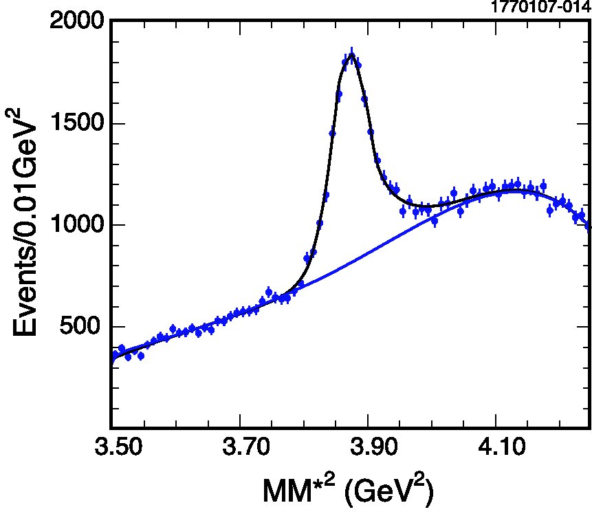 Figure 1
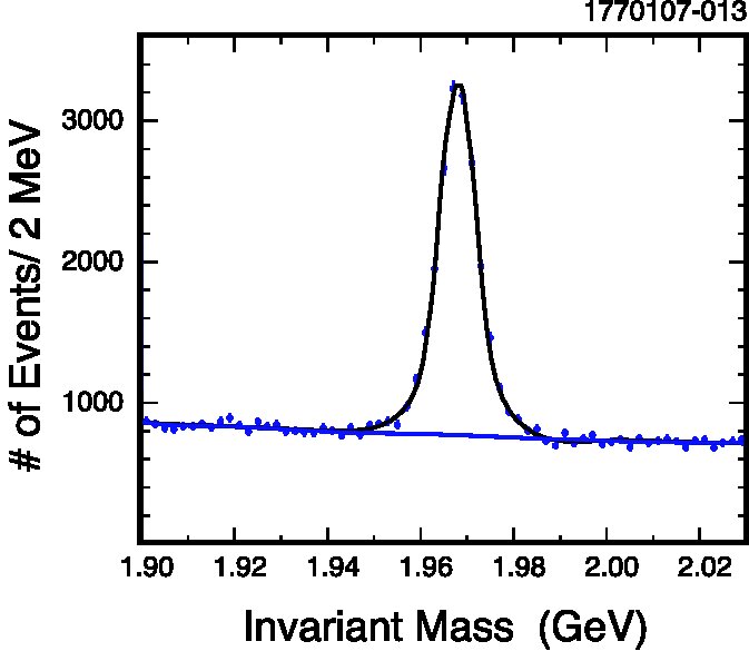 Figure 2
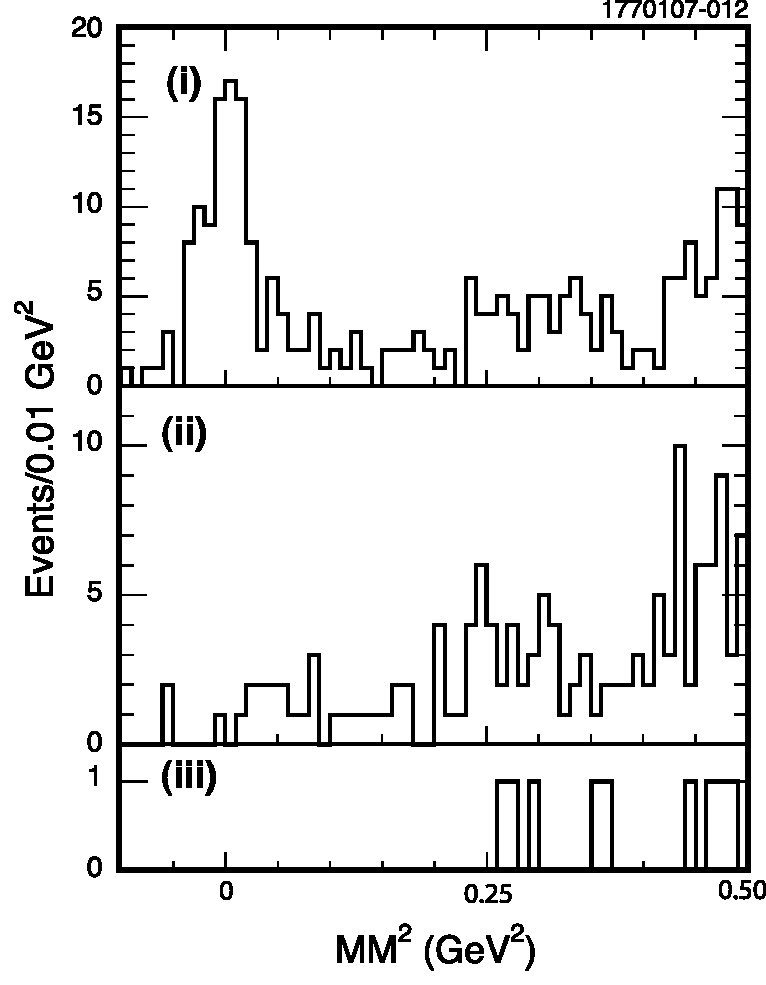 Figure 3
| Mode | Invariant Mass | MM∗2 | ||
|---|---|---|---|---|
| Signal | Bkgrnd | Signal | Bkgrnd | |
| 13871262 | 10850 | 8053 211 | 13538 | |
| 312279 | 1609 | 193388 | 2224 | |
| 4666 | 102497 | 3967 | ||
| 119646 | 409 | 79269 | 1052 | |
| 167874 | 1898 | 1050113 | 3991 | |
| 3654199 | 25208 | 2300187 | 15723 | |
| 203098 | 4878 | 1298130 | 5672 | |
| 4142281 | 20784 | 2195225 | 17353 | |
| Sum | 70302 | 18645426 | 63520 | |
| Source | (%) | case (i) | case (ii) | Sum |
|---|---|---|---|---|
| 8.2 | 0 | 0 | 0 | |
| 1.0 | 0.030.04 | 0.080.03 | 0.110.04 | |
| 6.4 | ||||
| 1.5 | 0.550.22 | 0.640.24 | 1.200.33 | |
| 1.0 | 0.370.15 | 0 | 0.370.15 | |
| Sum | 1.0 | 0.70.2 | 1.7 |
Peer Reviews
No public reviews on file for this paper yet. If you reviewed it on a platform where reviews are public (OpenReview, ICLR, NeurIPS, ICML), you can paste yours below so the community can read it here.
Videos
No videos yet. Explain this paper in a talk, walkthrough, or lecture? Add one.
CLEO Collaboration
Measurement of the Decay Constant
using
M. Artuso
S. Blusk
J. Butt
S. Khalil
J. Li
N. Menaa
R. Mountain
S. Nisar
K. Randrianarivony
R. Sia
T. Skwarnicki
S. Stone
J. C. Wang
Syracuse University, Syracuse, New York 13244
G. Bonvicini
D. Cinabro
M. Dubrovin
A. Lincoln
Wayne State University, Detroit, Michigan 48202
D. M. Asner
K. W. Edwards
P. Naik
Carleton University, Ottawa, Ontario, Canada K1S 5B6
R. A. Briere
T. Ferguson
G. Tatishvili
H. Vogel
M. E. Watkins
Carnegie Mellon University, Pittsburgh, Pennsylvania 15213
J. L. Rosner
Enrico Fermi Institute, University of Chicago, Chicago, Illinois 60637
N. E. Adam
J. P. Alexander
D. G. Cassel
J. E. Duboscq
R. Ehrlich
L. Fields
L. Gibbons
R. Gray
S. W. Gray
D. L. Hartill
B. K. Heltsley
D. Hertz
C. D. Jones
J. Kandaswamy
D. L. Kreinick
V. E. Kuznetsov
H. Mahlke-Krüger
D. Mohapatra
P. U. E. Onyisi
J. R. Patterson
D. Peterson
J. Pivarski
D. Riley
A. Ryd
A. J. Sadoff
H. Schwarthoff
X. Shi
S. Stroiney
W. M. Sun
T. Wilksen
Cornell University, Ithaca, New York 14853
S. B. Athar
R. Patel
J. Yelton
University of Florida, Gainesville, Florida 32611
P. Rubin
George Mason University, Fairfax, Virginia 22030
C. Cawlfield
B. I. Eisenstein
I. Karliner
D. Kim
N. Lowrey
M. Selen
E. J. White
J. Wiss
University of Illinois, Urbana-Champaign, Illinois 61801
R. E. Mitchell
M. R. Shepherd
Indiana University, Bloomington, Indiana 47405
D. Besson
University of Kansas, Lawrence, Kansas 66045
T. K. Pedlar
Luther College, Decorah, Iowa 52101
D. Cronin-Hennessy
K. Y. Gao
J. Hietala
Y. Kubota
T. Klein
B. W. Lang
R. Poling
A. W. Scott
A. Smith
P. Zweber
University of Minnesota, Minneapolis, Minnesota 55455
S. Dobbs
Z. Metreveli
K. K. Seth
A. Tomaradze
Northwestern University, Evanston, Illinois 60208
J. Ernst
State University of New York at Albany, Albany, New York 12222
K. M. Ecklund
State University of New York at Buffalo, Buffalo, New York 14260
H. Severini
University of Oklahoma, Norman, Oklahoma 73019
W. Love
V. Savinov
University of Pittsburgh, Pittsburgh, Pennsylvania 15260
O. Aquines
A. Lopez
S. Mehrabyan
H. Mendez
J. Ramirez
University of Puerto Rico, Mayaguez, Puerto Rico 00681
G. S. Huang
D. H. Miller
V. Pavlunin
B. Sanghi
I. P. J. Shipsey
B. Xin
Purdue University, West Lafayette, Indiana 47907
G. S. Adams
M. Anderson
J. P. Cummings
I. Danko
D. Hu
B. Moziak
J. Napolitano
Rensselaer Polytechnic Institute, Troy, New York 12180
Q. He
J. Insler
H. Muramatsu
C. S. Park
E. H. Thorndike
F. Yang
University of Rochester, Rochester, New York 14627
Abstract
We measure the decay constant using the channel, where the designates either a or a , when the . Using both measurements we find . Combining with our previous determination of , we compute the ratio . We compare with theoretical estimates.
pacs:
13.20.Fc, 13.66.Bc
††preprint:
CLNS 07/1989
CLEO 07-01
To extract precise information on the size of CKM matrix elements from and mixing measurements the ratio of “decay constants,” that are related to the heavy and light quark wave-function overlap at zero separation, must be well known formula-mix . Recent measurement of mixing by CDF CDF has shown the urgent need for precise numbers. Decay constants have been calculated for both and mesons using several methods, including lattice QCD Davies . Here we present the most precise measurement to date of , and combined with our previous determination of our-fDp ; DptomunPRD , we find .
In the Standard Model (SM) purely leptonic decay proceeds via annihilation through a virtual . The decay rate is given by Formula1
[TABLE]
where is the mass, is the lepton mass, is the Fermi constant, and is a CKM matrix element with a value of 0.9738 PDG .
In this Letter we report measurements of both and , when (). More details are given in a companion paper PRD . The ratio predicted in the SM via Eq. 1 depends only on well-known masses, and equals 9.72; any deviation would be a manifestation of new physics as it would violate lepton universality Hewett . New physics can also affect the expected widths; any undiscovered charged bosons would interfere with the SM Akeroyd .
The CLEO-c detector CLEODR is equipped to measure the momenta of charged particles, identify them using and Cherenkov imaging (RICH) fakes , detect photons and determine their directions and energies. We use 314 pb*-1* of data produced in collisions using CESR near 4.170 GeV. Here the cross-section for our analyzed sample, +, is 1 nb. Other charm production totals 7 nb poling , and the underlying light-quark “continuum” is 12 nb. We fully reconstruct one as a “tag,” and examine the properties of the . (Charge conjugate decays are used.) Track selection, particle identification, , , and criteria are the same as those described in Ref. our-fDp , except that RICH identification now requires a minimum momentum of 700 MeV/.
Tag modes are listed in Table 1. For resonance decays we select intervals in invariant mass within 10 MeV of the known mass for , 10 MeV for , 100 MeV for , and 150 MeV for . We require tags to have momentum consistent with coming from production. The distribution for the mode (44% of all the tags) is shown in Fig. 1.
To select tags, we first fit the invariant mass distributions to the sum of two Gaussians centered at . The r.m.s. resolution () is defined as , where and are the individual widths and is the fractional area of the first Gaussian. We require the invariant masses to be within ( for the mode) of . We have a total of 31302472 tag candidates. Then we add a candidate that satisfies our shower shape requirement. Regardless of whether or not the forms a with the tag, for real events, the missing mass squared, MM*∗2*, recoiling against the and the tag should peak at . We calculate
[TABLE]
where () is the center-of-mass energy (momentum), () is the energy (momentum) of the fully reconstructed tag, () is the energy (momentum) of the additional . We use a kinematic fit that constrains the decay products of the to and conserves overall momentum and energy. All ’s in the event are used, except for those that are decay products of the tag.
The MM*∗2* distribution from tags is shown in Fig. 2. We fit all the modes individually to determine the number of tag events. This procedure is enhanced by having information on the shape of the signal function. We use fully reconstructed events, and examine the signal shape when one is ignored. The signal is fit to a Crystal Ball function taunu , which determines and the shape of the tail. Though varies somewhat between modes, the tail parameters don’t change, since they depend on beam radiation and energy resolution.
Fits of MM*∗2* in each mode when summed show 18645426 events within a interval (see Table 1). There is a small enhancement of % in our ability to find tags in (or ) events (tag bias) as compared with generic events. Additional systematic errors are evaluated by changing the fitting range, using 4th and 6th order Chebychev background polynomials, and allowing the parameters of the tail of the fitting function to float, leading to an overall systematic uncertainty of 5%.
Candidate events are required to have only a single additional track oppositely charged to the tag with an angle 35.9*∘* with respect to the beam line. We also require that there not be any neutral energy cluster detected of more than 300 MeV, which is especially useful to reject and decays. Since here we are searching for events in which there is a single missing , the missing mass squared, MM2, should peak at zero:
[TABLE]
where () are the energy (momentum) of the candidate track.
We also make use of a set of kinematical constraints and fit each event to two hypotheses: (1) the tag is the daughter of a and (2) the decays into . The kinematical constraints, in the center-of-mass frame, are In addition, we constrain the invariant mass of the tag to . This gives a total of 7 constraints. The missing four-vector needs to be determined, so we are left with a three-constraint fit. We perform an iterative fit minimizing . To eliminate systematic uncertainties that depend on understanding the absolute scale of the errors, we do not make a cut but simply choose the and the decay sequence in each event with the minimum .
We consider three separate cases: (i) the track deposits 300 MeV in the calorimeter, characteristic of a non-interacting pion or a ; (ii) the track deposits 300 MeV in the calorimeter, characteristic of an interacting pion; or (iii) the track satisfies our electron selection criteria. The separation between muons and pions is not complete. Case (i) contains 99% of the muons but also 60% of the pions, while case (ii) includes 1% of the muons and 40% of the pions DptomunPRD . Case (iii) does not include any signal but is used for background estimation. For cases (i) and (ii) we insist that the track not be identified as an electron or a kaon. Electron candidates have a match between the momentum measured in the tracking system and the energy deposited in the CsI calorimeter, and and RICH measurements consistent with this hypothesis.
For the final state the MM2 distribution is modeled as the sum of two Gaussians centered at zero. A Monte Carlo (MC) simulation of the MM2 shows =0.025 GeV2 after the fit. We check the resolution using the mode. We search for events with at least one additional track identified as a kaon using the RICH detector, in addition to a tag. The MM2 resolution is 0.025 GeV2 in agreement with the simulation.
In the final state, the extra missing results in a smeared MM2 distribution that is almost triangular in shape starting near -0.05 GeV2, peaking near 0.10 GeV2, and ending at 0.75 GeV2.
The MM2 distributions from data are shown in Fig. 3. The overall signal region is -0.05 MM. The upper limit is chosen to prevent background from and final states. The peak in Fig. 3(i) is due to . Below 0.20 GeV2 in both (i) and (ii) we have events. The specific signal regions are: for , GeV2, corresponding to ; for , in case (i) GeV2 and in case (ii) GeV2. In these regions we find 92, 31, and 25 events, respectively.
We consider backgrounds from two sources: one from real decays and the other from the background under the single-tag signal peaks. For the latter, we estimate the background from data using side-bands of the invariant mass, shown in Fig. 1. For case (i) we find 3.5 (properly normalized) background events in the region and 2.5 backgrounds in the region; for case (ii) we find 3 events. Our total background estimate summing over all of these cases is 9.02.3 events.
The background from real decays is evaluated by identifying specific sources. For the only possible background is . Using a 195 pb*-1* subsample of our data, we limit the branching fraction as at 90% C.L. PRD . This low rate coupled with the extra veto yields a negligible contribution. The real backgrounds for are listed in Table 2. Using the SM expected ratio of decay rates we calculate a contribution of 7.4 events.
The event yield in the signal region, (92), is related to the number of tags, , the branching fractions, and the background (3.5) as
[TABLE]
where (80.1%) includes the efficiencies (77.8%) for reconstructing the single charged track including final state radiation, (98.3)% for not having another unmatched cluster in the event with energy greater than 300 MeV, and the correction for the tag bias (4.8%); (91.4%) is the product of the 99.0% calorimeter efficiency and the 92.3% acceptance of the MM2 cut of MM GeV2; (7.6%) is the fraction of events contained in the signal window (13.2%) times the 60% acceptance for a pion to deposit less than 300 MeV in the calorimeter. Using ) of (10.900.07)% PDG , the ratio of the to widths is 1.059; we find:
[TABLE]
We can also sum the and contributions for . Equation Measurement of the Decay Constant using still applies. The number of signal and background events changes to 148 and 10.7, respectively. becomes 96.2%, and increases to 45.2%. The effective branching fraction, assuming lepton universality, is
[TABLE]
The systematic errors on these branching fractions are dominated by the error on the number of tags (5%). Other errors include: (a) track finding (0.7%), determined from a detailed comparison of the simulation with double tag events where one track is ignored; (b) the error due to the requirement that the charged track deposit no more than 300 MeV in the calorimeter (1%), determined using two-body decays DptomunPRD ; (c) the veto efficiency (1%), determined by extrapolating measurements on fully reconstructed events. Systematic errors arising from the background estimates are negligible. The total systematic error for Eq. 4 is 5.2%, and is 5.1% for Eq. 5 as (b) doesn’t apply here.
We also analyze the final state independently. For case (i) we define the signal region to be the interval 0.05MM0.20 GeV2, while for case (ii) -0.05MM0.20 GeV2. The upper limit on MM2 is chosen to avoid background from the tail of the peak. The fractions of the MM2 range accepted are 32% and 45% for case (i) and (ii), respectively.
We find 31 [25] events in the signal region with a background of 3.5 [5.1] events for case (i) [(ii)]. The branching fraction, averaging the two cases is
[TABLE]
where the systematic error includes a contribution of 0.06% from the uncertainty on . We measure for the ratio of to rates using Eq. 4. Here the systematic error is dominated by the uncertainty on the minimum ionization cut. We also set an upper limit of at 90% C.L. Both of these results are consistent with SM predictions and lepton universality.
We perform an overall check of our procedures by measuring . We compute the MM2 (Eq. 2) using events with an additional charged track identified as a kaon. These track candidates have momenta of approximately 1 GeV/; here the RICH has a pion to kaon fake rate of 1.1% with a kaon detection efficiency of 88.5% fakes . For this study, we do not veto events with extra charged tracks, or ’s, because of the presence of the . We determine This method gives a result in good agreement with preliminary CLEO-c results using double tags of % Peter ; these results are not independent.
We also performed the entire analysis on a MC sample that is 4 times larger than the data sample. The input branching fraction is 0.5% for and 6.57% for , while our analysis measured (0.5140.027)% for the case (i) signal and (0.5210.024)% for and combined.
Using from Eq. 5, and Eq. 1 with a lifetime of (5007) PDG , we extract
[TABLE]
We combine with our previous result MeV our-fDp , and find
[TABLE]
Lattice QCD predictions for and the ratio have been summarized by Onogi Onogi . Our measurements are consistent with most calculations; examples are unquenched Lattice that predicts MeV and for the ratio Lat:Milc , while a recent quenched prediction gives MeV and Lat:Taiwan . There is no evidence yet for any suppression in the ratio due to the presence of a virtual charged Higgs Akeroyd .
The CLEO-c determination of is the most accurate to date and consistent with other measurements PDG ; PRD . It also does not rely on the independent determination of any normalization mode (e.g. ). (We note that a preliminary CLEO-c result using , Moscow is consistent with these results.)
We gratefully acknowledge the effort of the CESR staff in providing us with excellent luminosity and running conditions. This work was supported by the A.P. Sloan Foundation, the National Science Foundation, the U.S. Department of Energy, and the Natural Sciences and Engineering Research Council of Canada.
The reference list from the paper itself. Each links out to its DOI / PubMed record.
- 1(1) G. Buchalla, A. J. Buras and M. E. Lautenbacher, Rev. Mod. Phys. 68 , 1125 (1996).
- 2(2) A. Abulencia et al. (CDF), Phys. Rev. Lett. 97 , 242003 (2006). See also V. Abazov et al. (D 0), Phys. Rev. Lett. 97 , 021802 (2006).
- 3(3) C. Davies et al. , Phys. Rev. Lett. 92 , 022001 (2004).
- 4(4) M. Artuso et al. (CLEO), Phys. Rev. Lett. 95 , 251801 (2005).
- 5(5) G. Bonvicini et al. (CLEO) Phys. Rev. D 70 , 112004 (2004).
- 6(6) D. Silverman and H. Yao, Phys. Rev. D 38 , 214 (1988).
- 7(7) W.-M. Yao et al. , J. Phys. G 33 , 1 (2006).
- 8(8) T. K. Pedlar et al. (CLEO), ar Xiv:0704.0437[hep-ex], submitted to Phys. Rev. D .