Spectropolarimetric observations of the Ca II 8498 A and 8542 A lines in the quiet Sun
A. Pietarila, H. Socas-Navarro, T. Bogdan

TL;DR
This study presents spectropolarimetric observations of Ca II infrared triplet lines in the quiet Sun, revealing complex magnetic and dynamic behaviors that differ from simulations, especially in magnetic topology and wave activity.
Contribution
It provides new observational insights into the magnetic and dynamic properties of the Ca II lines in the quiet Sun, highlighting differences from high plasma-beta simulations.
Findings
Stokes V profiles often differ between the two lines despite close formation regions.
Magnetic topology influences Stokes V shape more than wave phase in the network.
Oscillatory behavior and shock waves are prominent in the network, with significant Stokes V asymmetries.
Abstract
The Ca II infrared triplet is one of the few magnetically sensitive chromospheric lines available for ground-based observations. We present spectropolarimetric observations of the 8498 A and 8542 A lines in a quiet Sun region near a decaying active region and compare the results with a simulation of the lines in a high plasma-beta regime. Cluster analysis of Stokes V profile pairs shows that the two lines, despite arguably being formed fairly close, often do not have similar shapes. In the network, the local magnetic topology is more important in determining the shapes of the Stokes V profiles than the phase of the wave, contrary to what our simulations show. We also find that Stokes V asymmetries are very common in the network, and the histograms of the observed amplitude and area asymmetries differ significantly from the simulation. Both the network and internetwork show oscillatory…
Click any figure to enlarge with its caption.
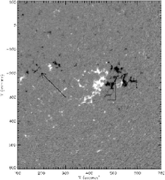 Figure 1
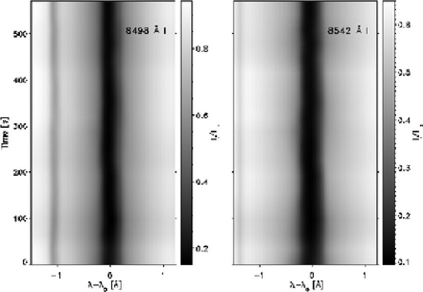 Figure 2
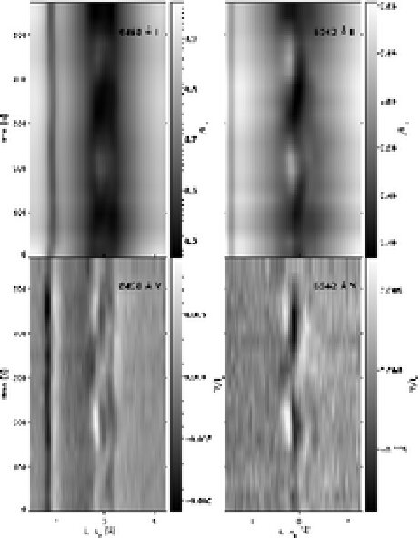 Figure 3
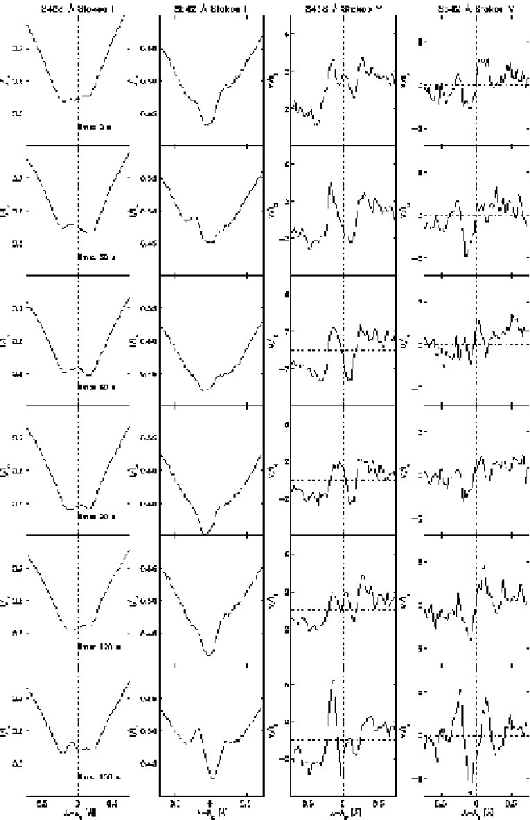 Figure 4
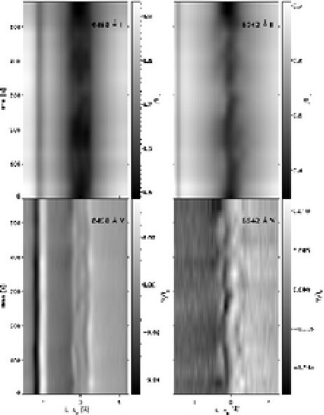 Figure 5
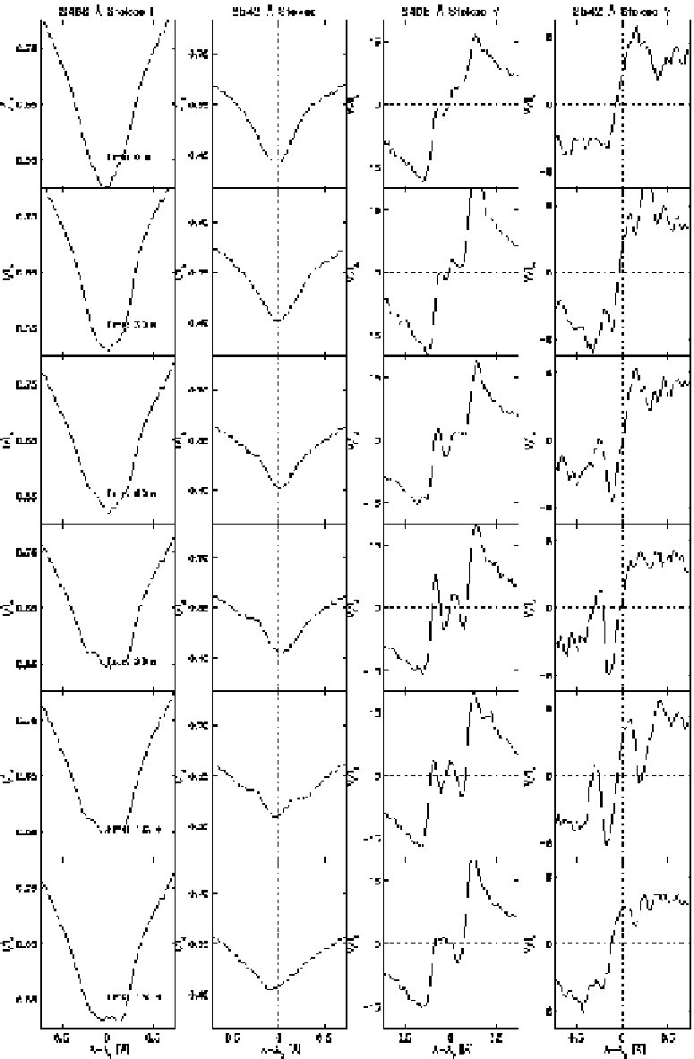 Figure 6
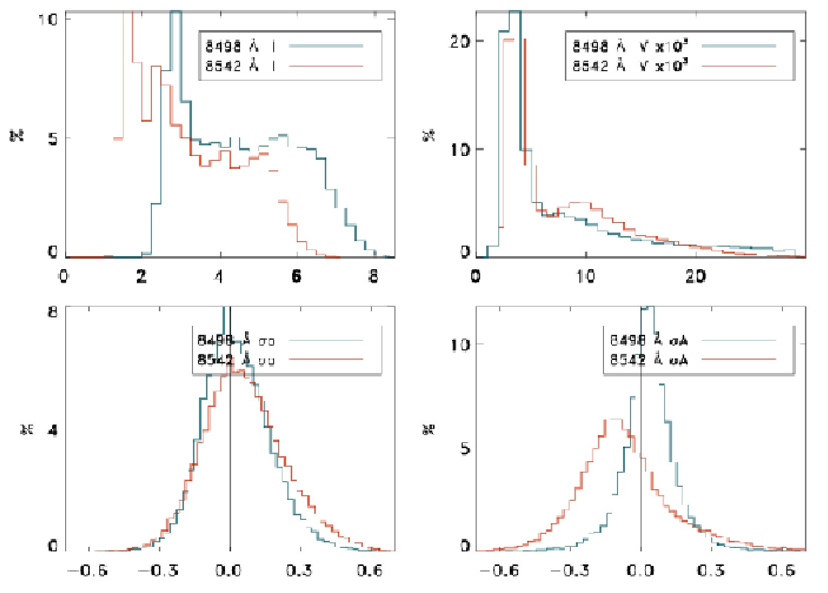 Figure 7
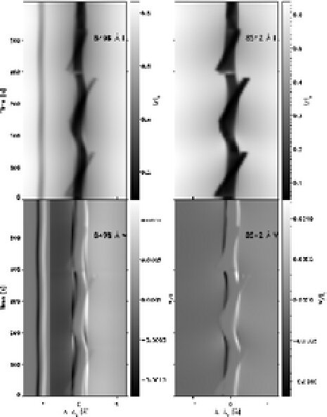 Figure 8
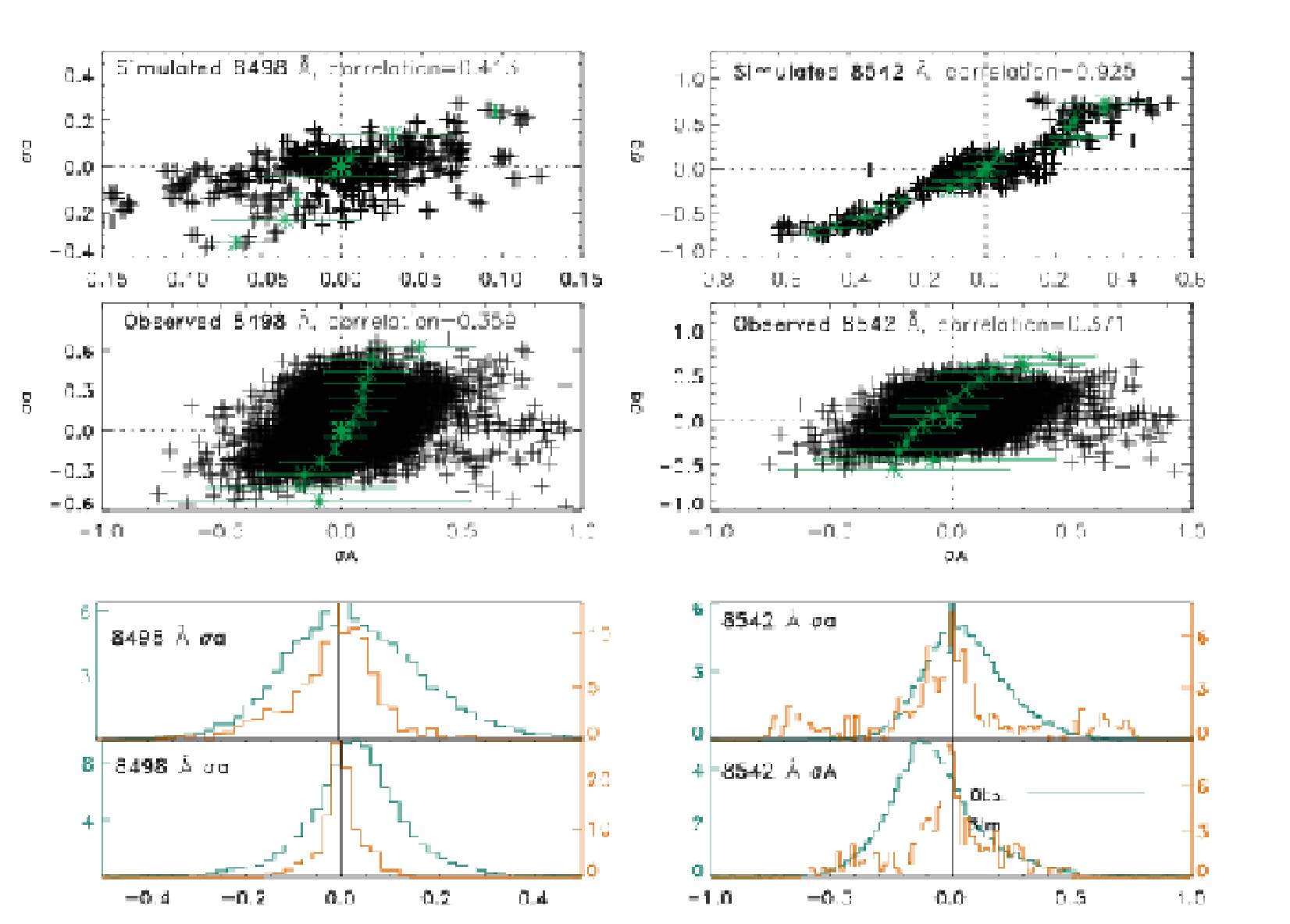 Figure 9
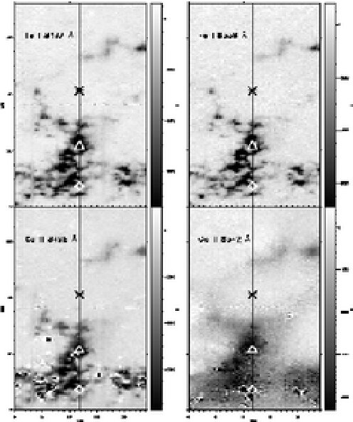 Figure 10
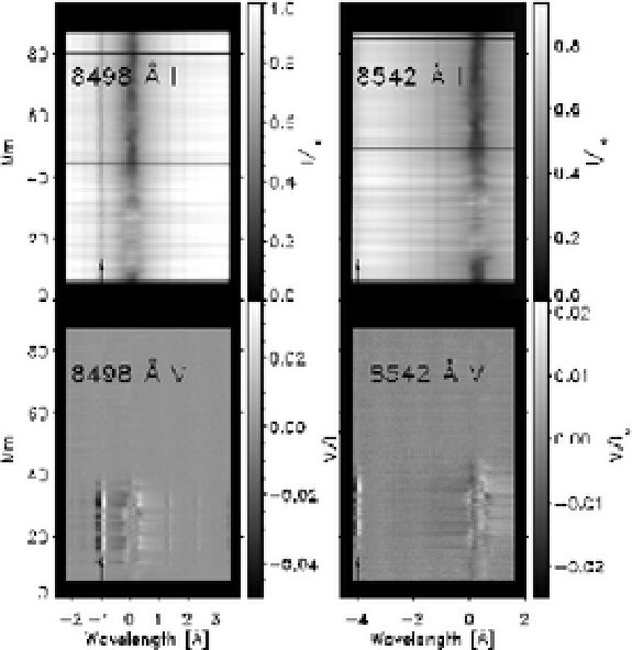 Figure 11
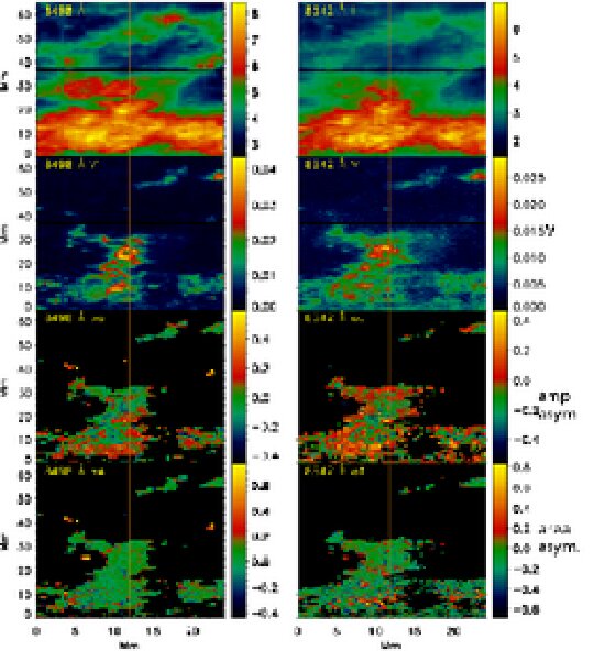 Figure 12
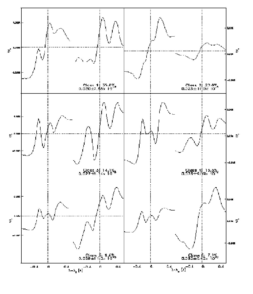 Figure 13
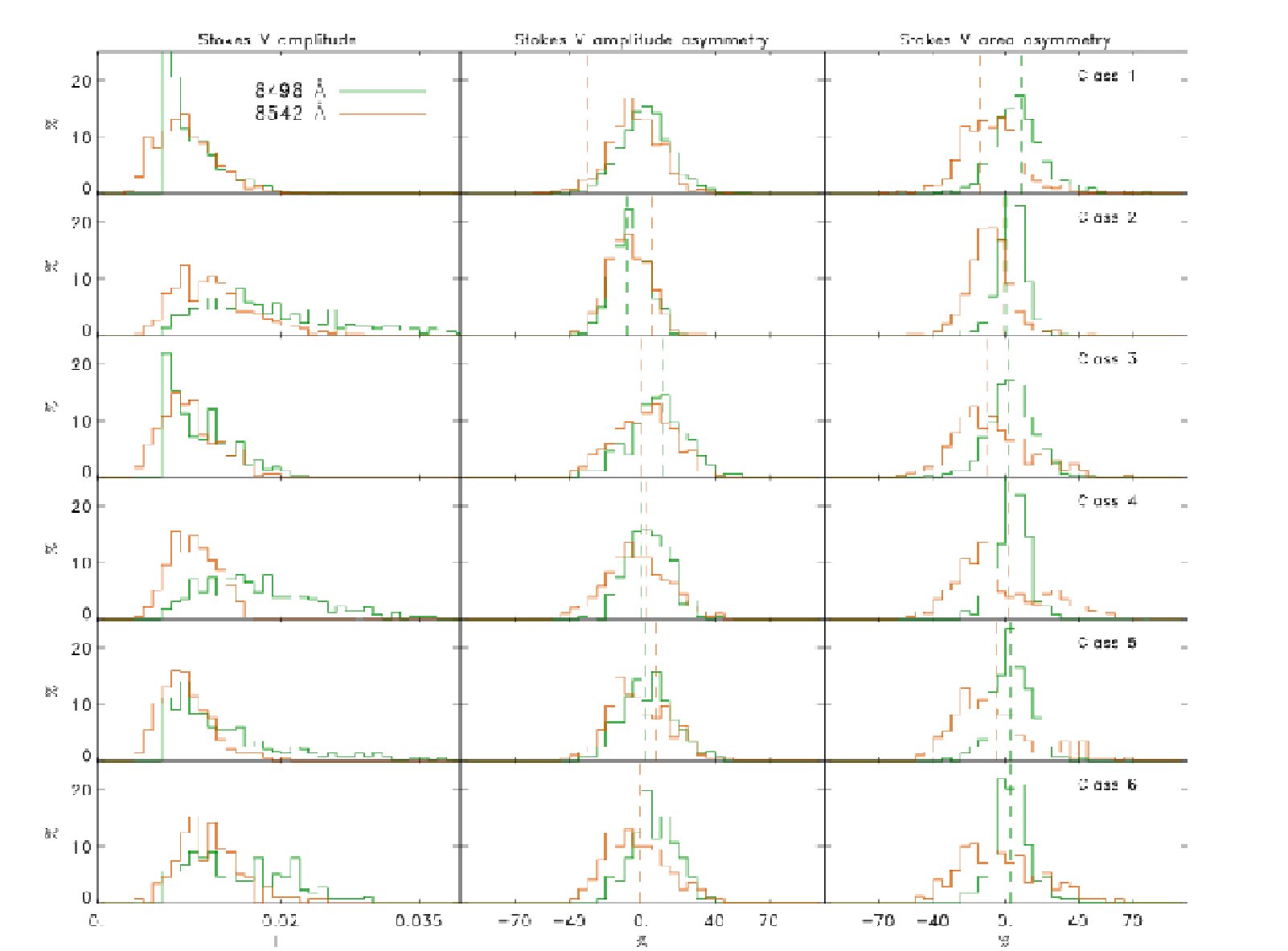 Figure 14
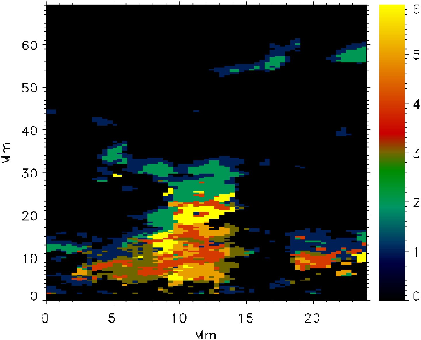 Figure 15
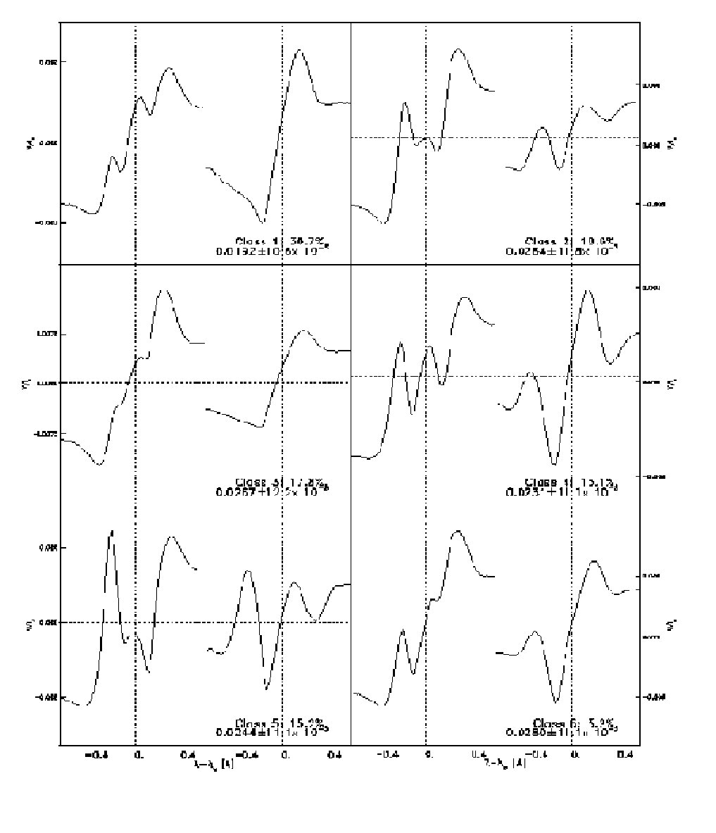 Figure 16
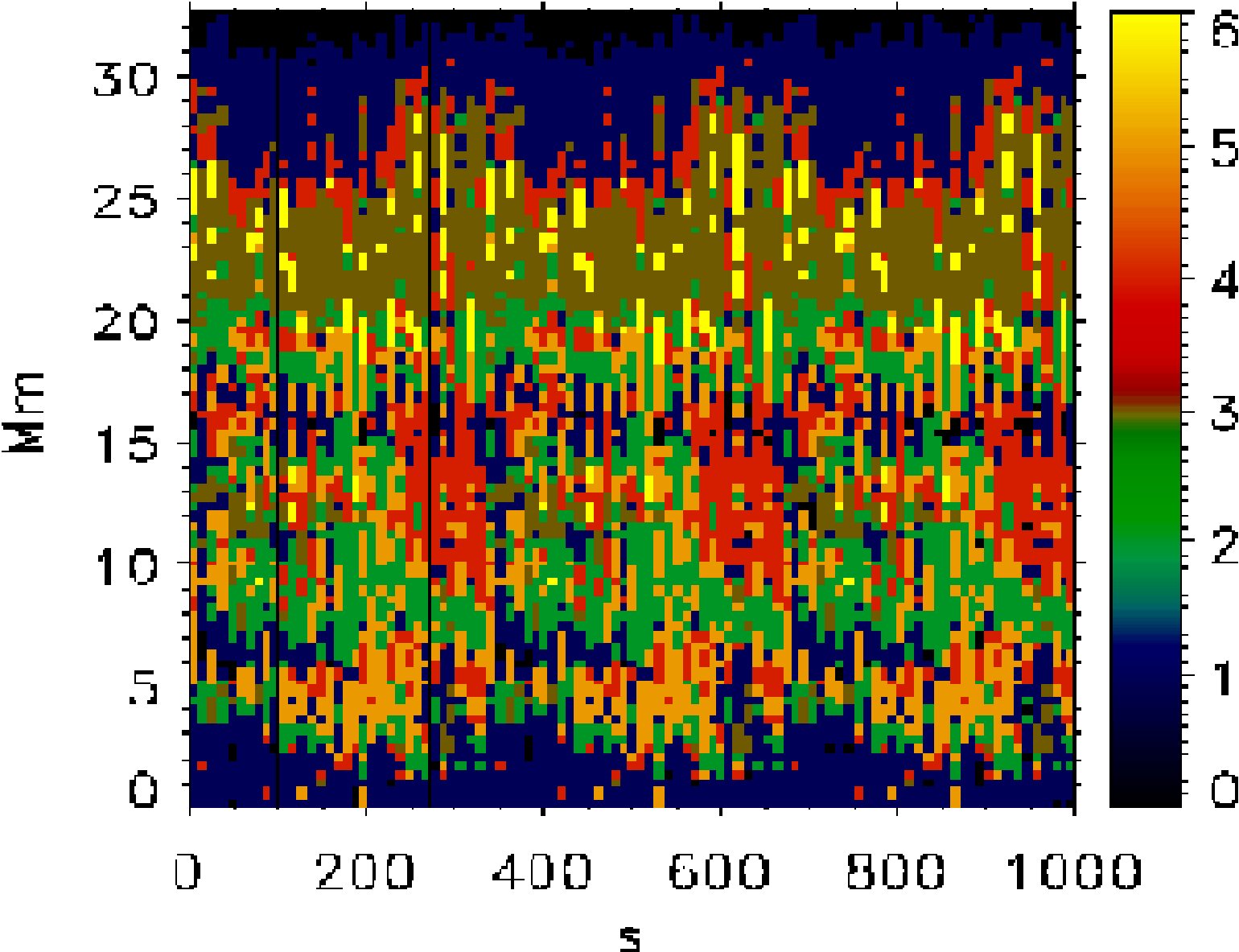 Figure 17
| 8498 Å | 8498 Å | 8498 Å | 8542 Å | 8542 Å | 8542 Å | |
|---|---|---|---|---|---|---|
| (%) | (%) | mean (%) | (%) | (%) | mean (%) | |
| a | 43.2 | 55.7 | 3.1 | 36.6 | 61.4 | 6.3 |
| A | 35.5 | 64.5 | 3.3 | 69.7 | 30.3 | -6.8 |
Peer Reviews
No public reviews on file for this paper yet. If you reviewed it on a platform where reviews are public (OpenReview, ICLR, NeurIPS, ICML), you can paste yours below so the community can read it here.
Videos
No videos yet. Explain this paper in a talk, walkthrough, or lecture? Add one.
Spectropolarimetric observations of the Ca II 8498 Å and 8542 Å lines in the quiet Sun
A. Pietarila11affiliation: Institute of Theoretical Astrophysics, University of Oslo, P.O.Box 1029 Blindern, N-0315 Oslo, Norway , H. Socas-Navarro
High Altitude Observatory, National Center for Atmospheric Research22affiliation: The National Center for Atmospheric Research (NCAR) is sponsored by the National Science Foundation. , 3080 Center Green, Boulder, CO 80301, USA
T. Bogdan
Space Environment Center, National Oceanic and Atmospheric Administration, 325 Broadway, Boulder, CO 80305, USA
Abstract
The Ca II infrared triplet is one of the few magnetically sensitive chromospheric lines available for ground-based observations. We present spectropolarimetric observations of the 8498 Å and 8542 Å lines in a quiet Sun region near a decaying active region and compare the results with a simulation of the lines in a high plasma- regime. Cluster analysis of Stokes profile pairs shows that the two lines, despite arguably being formed fairly close, often do not have similar shapes. In the network, the local magnetic topology is more important in determining the shapes of the Stokes profiles than the phase of the wave, contrary to what our simulations show. We also find that Stokes asymmetries are very common in the network, and the histograms of the observed amplitude and area asymmetries differ significantly from the simulation. Both the network and internetwork show oscillatory behavior in the Ca II lines. It is stronger in the network, where shocking waves, similar to those in the high- simulation, are seen and large self-reversals in the intensity profiles are common.
Subject headings:
polarization, Sun: chromosphere, waves
1. Introduction
Our understanding of solar magnetic fields outside active regions has increased significantly during the last years. This is due to new and better instrumentation (e.g., THEMIS, Paletou & Molodij 2001; VSM on SOLIS, Keller & The Solis Team 2001; Swedish Solar Telescope, Scharmer, Bjelksjo, Korhonen, Lindberg, & Petterson 2003; Solar Optical Telescope on Hinode, Shimizu 2004; and SPINOR, Socas-Navarro et al. 2006), better diagnostic techniques (see for example Bellot Rubio 2006 for a review on inversion techniques) and advanced numerical simulations (Stein & Nordlund 2006 and references therein). A large portion of the work has focused on photospheric magnetic fields. Only now we are starting to have adequate tools for investigating chromospheric magnetism in more detail. (For a review of chromospheric magnetic fields see Lagg (2005)). This is not surprising considering the numerous difficulties in observing chromospheric magnetic fields, interpreting the data, and performing realistic MHD simulations.
There are two different sets of lines that are often used for chromospheric spectropolarimetry, the He I infrared (IR) triplet at 10830 Å, and the Ca II IR triplet at 8500 Å. Both line sets have their advantages and disadvantages. The He I lines are formed over a relatively thin layer, and therefore observations can be inverted using a simple Milne-Eddington model. The drawback is that while the formation range is fairly narrow, the precise formation height remains uncertain, and the Milne-Eddington inversions do not give any information on the atmospheric gradients. The lines are also sensitive to the Paschen-Back effect, which must be included in the inversion code (Socas-Navarro et al., 2004). Furthermore, simulating the He I lines is difficult since coronal irradiation has a non-negligible effect on their formation (Andretta & Jones, 1997). In contrast, the formation of the Ca II IR lines is fairly well understood (Lites et al., 1982). The broad Ca II lines sample a large region of the atmosphere, from the photosphere to the lower chromosphere. However, the Ca II lines are formed in nonLTE, making inversions considerably more cumbersome.
Several investigations using the Ca II IR lines have studied intensity and velocity oscillations in the quiet Sun (e.g. Lites et al. 1982; Deubner & Fleck 1990) or, alternatively, magnetic fields in active regions (e.g. Socas-Navarro et al. 2000a). In both cases the lines have proven useful as diagnostics of the solar chromosphere. In this paper we present results of spectropolarimetric observations of two of the lines in an enhanced network region. We have both spatial maps and time series data. The observations show that the Ca II lines are formed in a very interesting region, namely the region where the atmosphere is transforming from a plasma dominated () to a magnetic field dominated () regime in terms of dynamic force balance. Wave propagation is clearly seen in the highly dynamic magnetic regions, whereas the weakly magnetic internetwork is found to be less variable. Interestingly, the two Ca II lines exhibit significant differences even though in calculations they are formed fairly close together. The importance of gradients in the chromospheric network is clearly demonstrated by the prevalence of asymmetric Stokes profiles in the data.
The paper is arranged as follows: in § 2 the data and their reduction are addressed. Results of analyzing the data using different approaches are presented in § 3. We performed cluster analyses on the Stokes profiles to classify them and to describe spatial patterns seen in the data. Statistics, such as profile amplitudes and asymmetries, are presented. The time dependent behavior of the lines in different network and internetwork regions is also discussed. In § 4 the observations are compared to simulations of the lines in a high plasma- regime (Pietarila et al. 2006, hereafter P06). Finally, in § 5 the main results are summarized and discussed.
2. Observations and data reduction
The Spectro-Polarimeter for INfrared and Optical Regions (SPINOR, Socas-Navarro et al. 2006) at the Dunn Solar telescope, Sacramento Peak Observatory, was used to observe two of the Ca II infrared triplet lines at 8498 Å and 8542 Å, as well as two photospheric Fe I lines at 8497 Å and 8538 Å. The setup included several other lines but because of computer problems only data from the two Ca lines which used the ASP TI TC245 cameras were recorded fully. The data have 256 points in both the wavelength and spatial position with a typical noise level of (1 deviation from the mean) and a spectral sampling of 25 mÅ. The pixel height corresponds to 0.38 arcseconds on the solar surface along the slit. We observed a quiet Sun region near disk center at S17.3 W32.1 on May 19, 2005 at 14:14 UT. An MDI-magnetogram of the region is shown in Figure 1. The slit was positioned in the vicinity of a decaying active region, AR10763, but avoided flux concentrations from the active region (i.e., plages). A time series consisting of 99 time steps of short scans (3 slit positions), with a spacing of 0.375 arcseconds each, was acquired during variable seeing conditions. The cadence is 10 seconds (i.e., a given slit position was repeated every 30 s). The time series was followed by a 63 step raster centered around the position where the slit was during the time series. The raster step size was 0.375 arcseconds. Adaptive optics (AO, Rimmele 2000) were used during the observing sequence but the compromised seeing conditions did not allow for continuous locking onto granulation. This caused the slit to jump occasionally, making the longest period with a stationary slit in the time series 17 time steps (8.5 min). The spatial resolution varied during the sequences being at best less than an arc second, but on average a factor of two worse.
Standard procedures for flat field and bias were used for the data reduction. Instrumental polarization was removed using the available calibration data, as explained in Socas-Navarro et al. (2006). No absolute wavelength calibration was attempted because no suitable telluric lines are present. Instead a wavelength calibration using spatial pixels devoid of magnetic field was done by fitting the average spectrum to the Kitt Peak FTS-spectral atlas (Neckel & Labs, 1984). The FTS atlas was also used to find the normalization factor for the intensities to the quiet Sun continuum intensities. Because of detector flatfield residuals and prefilter shape, the continua in the raw data from both detectors are tilted. The tilts were removed a posteriori by subtracting a linear fit () obtained by matching the continuum intensity levels to those of the FTS atlas.
The data were analyzed using both the raster and time series for statistical purposes. The period when the slit was stationary on the solar disk was used to study the time-dependent behavior of the lines. Because of the short length of this period, we do not present any Fourier analysis of the data. To make a classification of Stokes V profile morphologies, we did cluster analyses based on a Principal Component Analysis (PCA) in a similar manner as the work of Sánchez Almeida & Lites (2000) and Khomenko et al. (2003) for photospheric lines. We computed amplitudes for Stokes and profiles. Because the Ca line intensity profiles often exhibit strong self-reversals, no proxies for atmospheric velocities, such as lines’ centers of gravity or bisectors, are adequate. For those Stokes V profiles with amplitudes greater than , (i.e. ), amplitude and area asymmetries were also calculated.
The amplitude asymmetry of a Stokes V profile is defined by (Martínez Pillet, 1997):
[TABLE]
where and are the unsigned extrema of the blue and red lobes of the Stokes profile.
The area asymmetry of a Stokes profile is defined by (Martínez Pillet, 1997):
[TABLE]
where is the sign of the blue lobe. Because of the broad, deep lines and large velocities (compared with the photosphere) present in the chromosphere, the choice of the integration range for the area asymmetries is non-trivial for the Ca lines. We followed the same procedure as in P06. In the weak field regime the Stokes V profile is proportional to (strictly true only in the absence of atmospheric velocity and magnetic gradients). Inspection of the data showed that most of the observed Stokes profiles have roughly the same structures as the profiles. The intensity in the blue wing () of the line profile was matched with a point in the red wing () with the same intensity. The signal-to-noise in the intensity profiles is much higher than in the Stokes V profiles and also the slope is much steeper. This makes matching points with the same value more accurate in the intensity than in the Stokes V profiles. The selection of a wavelength to start the integration range was made by choosing a wavelength point that is far enough from the line core so that self-reversals are not an issue. In our data this point, , is at 600 mÅ from reference wavelength of line center. The same value was used in P06.
Magnetograms made from the 63 step scan are shown in Figure 2. The panels are in order of increasing formation height: Fe I 8497 Å, Fe I 8538 Å, Ca II 8498 Å and Ca II 8542 Å. The lower part of the slit was located above a flux concentration along the enhanced network and the upper part over an internetwork region with very little magnetic activity. The network becomes wider and more diffuse with increasing line formation height as described by Giovanelli (1980). Not all magnetic flux seen in the photosphere can be identified in the chromosphere and vice versa. However, interpreting the chromospheric magnetograms is difficult due to the self-reversed features in the cores of the Ca line Stokes profiles.
3. Results
In Figure 3, Stokes and spectra of the solar surface under the slit are shown for both Ca II lines as well as the two photospheric Fe I lines in the Ca lines’ wings (marked by arrows). Since the Fe I 8497 Å line is blended in the Ca line’s wing and the Fe I 8538 Å line is very close to the edge of the detector, no quantitative analysis is done for them. No signal above the noise was recorded in Stokes and so they will not be addressed in what follows. Residual vertical fringing caused by the polarization modulator is visible in the Stokes images. We chose not to try to remove the fringing since its’ amplitude is of the same order of magnitude as the noise.
The network, present in the lower part of the slit, is associated with less absorption in the intensity profiles. Both Ca lines often show self reversals, which are usually stronger on the blue side of the line than in the red. The Stokes profiles of both Ca lines have large, extended wings. At times, the profiles may have both polarities present on the blue side of the core but in almost all cases the far blue wing of the profile has the same polarity (i.e., opposite sign) as the red wing. The Stokes and profiles of the chromospheric lines look distinctively different from the photospheric lines: the Ca lines have more structure, they are wider and exhibit more spatial variation than the photospheric Fe lines. Some differences are seen between the two Ca lines: the 8542 Å line is slightly broader, has more structure in the spectra and also stronger absorption than the 8498 Å line.
The internetwork region, present in the upper part of the slit, is mostly devoid of Stokes signal, and Stokes is more homogeneous than in the network. Self reversals are usually not seen in the profiles. A small portion of the internetwork region has structures in Stokes that are similar to those seen in the magnetic region: Stokes is brighter than in the surrounding areas and the profiles show some self reversals. Closer inspection of the images reveals a visible, albeit a very small amplitude, Stokes signal.
The spatial patterns of Stokes and amplitudes and asymmetries in the two Ca lines (Figure 4) are fairly similar to one another. The network is clearly visible in the Stokes and amplitudes, though it is more diffuse in the 8542 Å line. There is a structure in the upper part of the map that is seen best in the 8498 Å intensity image. Parts of this structure appear also in both lines’ Stokes amplitude and asymmetry images. The edges of the network have more asymmetric Stokes profiles. This is seen clearly in the 8542 Å amplitude asymmetry.
Photospheric velocities can be estimated from the locations of the iron lines’ intensity minima. Except for a nearly constant offset caused by the convective down flows in the network, the internetwork and network regions have very similar spatial and temporal patterns.
3.1. Classification of the Stokes V profiles
To classify the shapes of the 8498 Å and 8542 Å Stokes profile pairs we used PCA, (Rees et al., 2000) and cluster analysis. The cluster analyses were performed separately for the map and the time series. Here we present a summary of the PCA procedure and cluster analysis for completeness.
With the PCA we are able to reduce the number of parameters needed to describe a given profile. Each profile, , ( is the number of wavelength points in the profile) is composed of a linear combination of eigenvectors , :
[TABLE]
where the are appropriate constants. The eigenvectors and constants for a given set of profiles are obtained from a singular value decomposition (SVD, Rees et al. 2000, Socas-Navarro et al. 2001) and form an orthonormal basis with eigenvectors:
[TABLE]
Not all eigenvectors contain the critical information needed to reproduce the profiles, some of the eigenvectors carry information about the noise pattern. We can therefore truncate the series expansion and use only a small number of eigenvectors and corresponding coefficients to reproduce a given profile. The PCA guarantees that when expansion of Eq. 3 is truncated at a given order , the amount of information in the lower orders is maximized.
We performed the SVD for the two 8498 Å and 8542 Å Stokes profiles separately. The resulting orthonormal bases, and also the cluster analysis, depend on the subset of profiles used to construct it. Because of this we included all Stokes profiles from pixels where the 8498 Å Stokes amplitude is above , altogether 13671 profiles. Visual inspection of the eigenvectors shows that the first 11 eigenvectors (approximately) contain relevant information about the actual shape of the profiles whereas the remainder are associated with the noise patterns.
The Stokes profile pairs, now described with 11 2 coefficients corresponding to the 11 2 eigenvectors instead of 102 (51 for each profile) wavelength points, were organized into a predefined number of clusters. Before doing this the vectors consisting of the 22 coefficients were standardized, i.e., no information of the absolute Stokes amplitudes is left, only the relative amplitudes of the 8498 Å and 8542 Å profiles. Based on the values of the coefficients, 6 cluster centers were identified using the -means method (MacQueen, 1967). It starts with random clusters, which through iterations are changed to minimize the variability within a cluster and maximize it between clusters. Each profile pair is then assigned to the nearest cluster center in the 22-dimensional Euclidean space. The choice of number of clusters used for the cluster analysis is non-trivial. Since each data point is described by 22 numbers we cannot visually distinguish patterns in the spatial distribution of the points. Instead the number of clusters was defined by trial and error, i.e. so that each profile type in the time series or map is represented and each cluster is still clearly distinct from one another. For each cluster a profile was constructed using the eigenvectors and the averaged 2 11 coefficients of all profiles belonging to that cluster.
Cluster analysis of the map shows the shapes of Stokes V profiles in network regions with different magnetic topologies, whereas the time series analysis describes how a set of profiles from a certain magnetic topology changes with time.
The results for the map are shown in Figure 5. Above each profile is the percentage of all profiles belonging to the cluster, the mean distance in the Euclidean space of the profiles to the cluster center, and the standard deviation of the mean. The smaller the distance to the cluster center, the more compact the cluster is and the better the cluster describes the profiles. The standard deviation is proportional to the spread of the distances in each cluster. In general, clusters with the least number of profiles belonging to them have larger mean distances.
Three points can be deduced from the figure. First, asymmetric profiles should be common. In fact, they appear to be more common than symmetric ones. Second, even though the two Ca lines are formed fairly close to one another (the 8498 Å line core optical depth is unity at about 1 Mm and the 8542 Å 0.2 Mm higher up in the radiation hydrodynamic simulations by Carlsson and Stein 1997), the 8498 Å and 8542 Å profiles in a given cluster are often clearly different from one another. Third, in all cluster profiles the far-red wings have the same polarity as the far-blue wings, indicating that the lower parts along the line-of-sight of the atmosphere, where the wings are formed, are dominated by a single magnetic polarity.
The clusters differ from one another in several different ways: the degree of asymmetry, and distinct relationships between the 8498 Å and 8542 Å line profiles, relative amplitudes, etc. However, quantitative measures, such as profile asymmetries, of the clusters do not necessarily represent the members of a given cluster very well. For example, the variation of Stokes amplitude asymmetries within a cluster is large and the mean is not necessarily the same as that of the cluster profile. The cluster analysis retrieves qualitative similarities and gives a basis for morphological classification, rather than representing quantitative similarities within the data. To illustrate this point, Figure 6 displays histograms of the clusters showing the Stokes amplitudes and asymmetries for all profiles belonging to a given cluster. Shown in Figure 7 is the spatial distribution of the clusters. The smallest network patches often consist of only cluster 1 and cluster 2 profiles. The middle of the largest network patch is a mixture of different clusters.
In most cases, the profiles at the edges of the network patches belong to cluster 1. This is the most common cluster consisting of 35.6 % of all the profile pairs in the map. The cluster 1 profiles are asymmetric, 8542 Å more so than 8498 Å, and they also have opposite signs of amplitude and area asymmetries. The amplitude histograms of profiles belonging to this cluster show that they have in general low amplitudes, as one might expect from profiles located at the edges of the network. The large amplitude asymmetry in the 8542 Å cluster profile is not seen in the observed profiles. In fact, only very few profiles exhibit such large asymmetries and there is only a slight tendency of the profiles having more often negative than positive amplitude asymmetries. The cluster area asymmetries are in better agreement with the observed profiles belonging to this cluster.
Regions of cluster 2 profiles are often located adjacent to patches of cluster 1 profiles. The cluster 2 profiles account for 20.0 % of all profile pairs in the map. The cluster profiles are fairly antisymmetric. This is seen in the observed profiles as well: the asymmetry histograms tend to be narrow and only slightly offset from zero. The relative amplitudes of the two cluster profiles are very different: the 8498 Å amplitude is a factor 3 larger. The disproportionality is not as large in the observed profiles though the amplitude histograms show that in general 8498 Å has a larger amplitude than 8542 Å. The range of observed amplitudes is considerably larger than in cluster 1.
Of the profile pairs in the map 14.1 % belong to cluster 3. Also, these profiles are often found in regions close to the network edges by the patches of cluster 1 profiles. Both cluster profiles have multiple lobes and are asymmetric, 8498 Å more in amplitude and 8542 Å in area. This is also seen in the histograms of the observed asymmetries. There is a strong emission feature on the blue side of the line in the 8498 Å cluster profile. It is weaker in the 8542 Å profile. The histograms for cluster 3 are nearly identical to those of cluster 1. This illustrates how cluster analysis based on PCA is captures the qualitative differences in the line profiles.
Cluster 4 consists of 13.5 % of the profile pairs. Most of the observed profiles belonging to this cluster are near to the middle of the largest network patches. The 8498 Å cluster profile is dominated by a strong emission feature in the blue lobe. This feature is not visible in the 8542 Å cluster profile. The overlap between the two lines’ amplitude histograms is fairly small. Also the cluster profiles show this difference in the relative amplitudes: 8542 Å has a significantly lower amplitude than 8498 Å. Except for the 8542 Å area asymmetry histogram, all histograms are centered around zero. The range of area asymmetries in the 8542 Å line is large and the distribution is skewed towards negative values. This trend in the 8542 Å area asymmetries is seen in several of the clusters.
The patches of profiles belonging to the fifth cluster (9.6 %) are also found in the less homogeneous middle regions of the network elements. The 8498 Å cluster profile has a factor 2 lower amplitude than 8542 Å. This is not seen in the amplitude histograms but there is a large overlap between the two histograms. The cluster profiles are fairly antisymmetric and also the histograms of observed profile asymmetries are centered around zero. The 8542 Å area asymmetry is again the exception: it is centered around a negative value.
Cluster 6 is the smallest cluster with 7.2 % of the profiles. Patches of cluster 6 profiles are located in regions with cluster 4 and 5 profiles. The 8498 Å cluster profile is very similar to that of cluster 5. Like cluster 5, the 8542 Å cluster 6 profile has a factor 2 larger amplitude and the amplitude histograms overlap nearly entirely. All the cluster 6 histograms are very similar to cluster 5. The major difference between the two is that there is very little structure in the 8542 Å line profile.
3.2. Time-dependent behavior
The cluster analysis results of the time series are shown in Figure 8, and the spatio-temporal distribution is captured in Figure 9. The clusters consist of profiles at rest with varying degrees of structure, and profiles where the blue side is in emission. While there are temporal changes in the clusters, there are no clear periodic patterns visible. Most slit positions have a preferred cluster or in some cases the slit position is dominated by two clusters. Positions where more than 2 clusters are dominant are rare.
Because the slit moved occasionally during the time series, no meaningful power spectra can be made from this data set. The time series data do however allow for a qualitative analysis of the time-dependent behavior. Comparing network and internetwork pixels reveals some interesting features: the network, especially in the intermediate flux regions, is very dynamic with propagating shock-like features and large self-reversals appearing frequently in both Stokes and . In comparison, the internetwork is less dynamic, intensity oscillations are present but they are much weaker than in the network. No structures indicating the presence of shocks, are seen in the internetwork profiles. In agreement with prior observations of chromospheric lines (e.g., Noyes 1967), any oscillation periods in the network appear to have a longer period than in the internetwork.
We now examine three different regions, namely an internetwork pixel, an intermediate flux network pixel, and a strong network pixel.
3.2.1 Internetwork
In Figure 10 the time evolution of a typical internetwork pixel is shown. The location of the pixel is marked by an asterisk in Figure 2. The data were taken when the slit was stationary. No Stokes signal above the noise level is seen in the pixel. The Stokes profiles of both Ca lines change periodically in width and position of the line center, but no self-reversals are seen. Also, the line-wing intensity shows some oscillations.
3.2.2 Intermediate flux network
The difference between the internetwork and network regions with intermediate flux (Fig. 11) is dramatic: the network region is much more dynamic, and highly asymmetric profiles, in both lines Stokes and , are seen. The time dependent behavior of the photospheric iron line is quite similar to what is seen in the internetwork.
The Stokes in both lines has a clearly oscillating behavior with bright, very asymmetric episodes followed by a darker, more symmetric episodes. The period for the oscillation is about 4 minutes, i.e. below that associated with the acoustic cutoff frequency (about 5.3 mHz). This may be caused by the presence of inclined magnetic fields can lower effectively the acoustic cutoff frequency (Bel & Leroy, 1977). The time evolution of the 8542 Å Stokes has a diagonal structure moving from blue to red. This indicates the presence of propagating compressible waves (Carlsson & Stein, 1997). The bright part, which corresponds to a large self-reversal, is clearly shifted towards the blue. This is seen in the 8498 Å line profiles as well, although these profiles tend to be more flat-bottomed. In general, the self-reversals and over all variation is larger in the blue wing than in the red. This is true for all slit positions which exhibit strong time-dependent behavior.
The Stokes image of the 8498 Å line also shows strong diagonal structures that coincide in time with the dark phases of Stokes . Inspection of individual profiles (Fig. 12) reveals a pattern of multiple lobes in the Stokes profiles. These lobes are on the blue side of the line core and their amplitudes and positions vary periodically in time resulting in the diagonal structure seen in the image. The lobes can be identified with the emission features seen in the Stokes profiles. The 8542 Å line Stokes image shows a pattern of a multi-lobed profiles whose amplitudes vary strongly in time. The large Stokes amplitude phase coincides with the bright, very asymmetric phase seen in the intensity profiles. The red wings always exhibit less structure and variation than the blue wings.
3.2.3 Strong network
Stokes and profiles seen in the strong network regions (Figs. 13 and 14) would appear at first glance to be a mixture of the less dynamic internetwork and the highly dynamic intermediate flux region. The Stokes profiles exhibit the same pattern of bright (more asymmetric) and dark (less asymmetric) phases as seen in the intermediate flux region. The difference between the two phases is however not as large: the amplitude of the self-reversals, especially in the 8542 Å intensity profiles, is much smaller than in the intermediate flux case.
The Stokes images resemble those of the intermediate flux region: some diagonal structures are seen, but they are weaker. The 8542 Å line Stokes profiles have a time varying amplitude but the profiles are not as asymmetric and they are not necessarily multi-lobed. The difference between the time-dependent behavior of the red and blue lobes of the profile, i.e. the red lobe varies less in time, is even more clear here than in the intermediate flux region.
3.3. Statistics
Histograms of the Stokes amplitude integrated over 250 mÅ around the line core for the two Ca lines are shown in the top-left panel of Figure 15. These histograms include both the map and time-series profiles. Because there are almost five times as many profiles in the time-series as there are in the map, the histograms are dominated by the time-series profiles. Both lines exhibit a wide range of values. Except for the peaks at low intensities, the histograms are fairly flat. The darkest (i.e. lowest core intensity or most absorption) amplitudes, are associated with the internetwork, and the brightest with the network.
Histograms of the Stokes amplitudes (top right panel of Fig. 15) peak at the same value in both lines, 0.003 , but the 8498 Å histogram tail decays more slowly. Since the 8498 Å line is formed slightly lower of the two and the lines are roughly equally sensitive to magnetic fields (effective Landé g factors are 1.07 and 1.10 for the 8498 Å and the 8542 Å lines, respectively), it is not surprising that the 8498 Å histogram has the longer tail.
Both lines’ Stokes amplitude asymmetry histograms (bottom left panel of Fig. 15) have very similar shapes and similar widths. There are more positive asymmetries in both lines: 56% in 8498 Å and 64 % in 8542 Å (Table 1). The mean amplitude asymmetries are also positive, and the 8542 Å mean asymmetry is two times larger. There are more negative amplitude asymmetries in the 8542 Å map than in the time series. Non-zero amplitude asymmetries indicate at least one of two things: the spatial pixels consist in most cases of at least two atmospheric components that are shifted relative to one another or that there are velocity and/or magnetic field gradients present in the atmosphere.
The area asymmetry histograms (bottom right panel of Fig. 15) of the two calcium lines repeat the pattern already seen in the cluster profiles: the 8542 Å histograms is centered around a negative value and the 8498 Å is centered at roughly zero, though the mean is slightly positive. The 8542 Å histogram is significantly wider than the 8498 Å histogram. A multi-component atmosphere alone cannot produce area asymmetries, so the existence of non-zero area asymmetries indicates the presence of velocity and possibly magnetic gradients in the atmosphere.
In the 8542 Å line 66 % of the profiles have negative area asymmetries whereas in the 8498 Å line the majority of the profiles, 64 %, have positive area asymmetries (Table 1). To better understand why the area asymmetry histograms of the lines are so different, we need to look at the components of the area asymmetry separately i.e. the sign of the blue lobe and the total area of the Stokes profile. One possible cause for the difference in the histograms might be that the distribution of signs of the blue lobe is different in the two lines. Closer inspection reveals that this is not the explanation. The vast majority of both lines, over 80 %, have a negative sign. (Here the sign is defined to be the sign of the local maximum or minimum amplitude of the blue lobe). A second possible explanation is that the is different in the two lines. This is found to be the case. The 8542 Å line has more profiles with a positive area and the 8498 Å has slightly more profiles with a negative area. (Note that the sign of the area asymmetry is the product of the sign of the blue lobe and the area; eq. 2.) The area of the Stokes profile is strongly affected by the emission features. These features, and their amplitudes, are related to the self-reversals seen in the Stokes profiles. The self-reversals are stronger on the blue side of the line core than on the red. In general, the blue lobes of the Stokes profiles have negative amplitudes and the effect of the emission features is then to reduce the amplitude, and in some cases, make it positive and this way reduce the overall negative area.
The effect of the emission features on the amplitude asymmetries is not as large because the amplitude will be affected only if the emission feature is located at the same wavelength as the maximum absolute amplitude. Also if the profile has a wide blue lobe, i.e., the wings contribute significantly, a local reduction in peak amplitude is counterbalanced by a comparable signal in the other parts of the blue lobe. The resulting profile will have nearly the same amplitude in the blue lobe as before, but the area will be reduced leading to a smaller, or even negative, area asymmetry. Since the self-reversals are larger in the 8542 Å line, this scenario is more likely to apply to it than the 8498 Å line.
Both lines’ area and amplitude asymmetries are found to be inversely proportional to the Stokes amplitudes. The scatter, especially in the 8542 Å line, is fairly large.
PCA also allows us to ensure that the determination of Stokes asymmetries is not dominated by noise. Reconstructing the profiles using only the 11 first eigenvectors (i.e., essentially noise-free profiles) and then computing the asymmetries reproduces the Stokes amplitude and asymmetry histograms. To test if the negative histogram peak in the 8542 Å line is an artifact caused by data reduction, we computed area asymmetries for the datasets, but after first removing the fringe pattern caused by the optics. This did not alter the area asymmetry histogram. Another artifact that could cause the offset is an incorrect subtraction of the tilt caused by the detector in the continuum intensity. To remove the offset in the histograms by means of changing the tilt causes a clearly visible lopsidedness in the Stokes I profiles. Lastly, to make sure that the choice of the integration range is not the cause of the offset, we used a constant bandwidth for area asymmetries and it also reproduces the 8542 Å area histogram offset. (Besides these issues, there are no other obvious artifacts that would cause the offset.) We therefore conclude that the offset is not caused by the fringing or incorrect subtraction of the tilt in the continuum intensity.
4. Comparison of observations with a high- simulation
In P06 we synthesized Stokes profiles for the Ca IR triplet lines in the high- regime. This was done by combining a radiation hydrodynamic code (see for example Carlsson & Stein 1997) with a weak magnetic field and using a nLTE Stokes inversion and synthesis code (Socas-Navarro et al., 2000b) to produce, based on snapshots of the simulation, a time series of the lines’ Stokes vectors. The simulation is driven by a photospheric velocity piston and its dynamics are dominated by upward propagating acoustic waves in a simple magnetic field topology. The simulation shows that the radiative transfer is very similar in all the Ca IR triplet lines. The differences between the line behaviors in the simulation are mainly due to the lines having slightly different formation heights and thus experiencing a difference in the amplitudes of the shocking waves: the higher the line is formed, the larger the amplitude of the passing wave is.
In the simulation there is no feedback from the magnetic fields on the dynamics and the waves are purely acoustic. The observations have limited spatial and temporal resolutions whereas the simulation is much better resolved.
4.1. Comparison of time dependent behavior
As the acoustic waves in the simulation propagate upwards and eventually form shocks, a time-varying pattern of disappearing and reappearing Stokes lobes is seen (Fig. 16). The pattern is strongest in the highest forming line, i.e. 8542 Å. Wave propagation is also seen in the Stokes profiles. There are no large self reversals or brightenings, instead the position of the line minimum changes periodically and forms a saw-tooth like pattern where the red shift takes more time than the blue shift phase.
If we first compare the simulated profiles to the internetwork observations (Fig. 10), we see that the strong signatures of shocks seen in the simulation are not present in the observations. In the simulation the Ca IR triplet is formed in a region where the waves are just beginning to shock. If the formation height of the lines or the shocks in the simulation is off, compared to the real Sun, by a small amount, even 50 km, the lines’ temporal evolution may look very different. Another possible explanation to why we see no strong indications of shocks is the temporal and/or spatial resolution: there may be several components oscillating out of phase relative to one another in a given resolution element. However, the photospheric velocities are very similar in the internetwork and network, but the network profiles show strong self-reversals. This suggests that spatial and temporal resolution alone cannot explain the lack of strong signatures of shocks in the internetwork.
Observations of the quiet Sun show varying degrees of oscillatory power (compare for example Lites et al. (1993) [Ca II H and K] or UV data of Judge et al. 2003, McIntosh & Judge 2001 and Wikstøl et al. 2000). This variation may be related to the local magnetic topology, especially to the possible existence of a magnetic canopy (McIntosh et al., 2003; Vecchio et al., 2006). The region observed here was less oscillatory than average but still not exceptionally quiet.
Both the simulated profiles and observed network profiles (Fig. 13) show time varying patterns where the Stokes and amplitudes change periodically. In the simulation the wave propagation manifests itself in the Stokes profiles most clearly as a shift of the line core and the saw-tooth shape of the time series. In the observations, waves cause the lines’ periodically varying self-reversals that result in alternating bright and dark phases. There are indications of diagonal structures in the observed Stokes images, but they are not nearly as clear as in the simulation. In the simulation the upward propagating waves cause the blue and red lobes of the Stokes profiles to disappear alternately. In contrast, the observed time varying pattern in Stokes looks more complicated: there is much more structure in the observed profiles, especially in the line cores, than in the simulation. This is related to the simulated profiles not exhibiting strong self-reversals as seen in the observations.
In the simulation, because of radiative cooling and expansion of the falling material, the down flows are in general cooler than the up flows. In the synthesized profiles this manifests itself by the red wings of the Stokes profiles showing less variations, though the difference with the blue wing is quite small. Similar behavior is also seen in the observations: the self-reversals are in general larger in the blue wing of the Stokes profiles and the red lobes of the Stokes profiles show clearly less variation.
4.2. Comparison of statistics and Stokes morphologies
In the simulation the magnetic field decays exponentially with height and therefore the Ca II Stokes amplitudes are significantly lower than the Fe I 8497 Å amplitude. In the observations the Ca and Fe line Stokes profiles have roughly the same amplitudes. This may be explained by the field decaying much slower with height in the observations, or by the filling factor in the observations being smaller in the photosphere than in the chromosphere.
Both Ca II lines’ observed Stokes profiles have a significant amount of signal in the wings. In the simulations only the 8498 Å line Stokes has extended wings with large amplitudes (Fig. 4 in P06). The amount of signal in the wings depends on the atmospheric magnetic field gradient. If there is no gradient the wings of all three Ca lines have very little signal. Whereas a model atmosphere with a constant field gradient produces profiles where all lines, 8498 Å the most, have some signal in the line wings and an exponential field produces profiles with the largest wings. Depending on where the gradient is located and how strong the field is, the Ca lines may or may not have similar Stokes profiles. Based on the profile shapes and relative amplitudes, it is obvious that the magnetic topology in the observations is different from the simulation.
Formation of area and amplitude asymmetries in the simulation is coupled. The correlation is especially strong in the 8542 Å line (upper row of Fig. 17). In the 8498 Å Stokes profiles the strong wings affect the asymmetries, and the correlation is weaker. The observed area and amplitude asymmetries of both lines show less correlation. This is at least partly because the observed profiles have more complex shapes than in the simulation.
The lower panels in Figure 17 show the Stokes asymmetry histograms for the simulation. The observed histograms are re-plotted to enable direct comparison. In the simulation both lines’ amplitude and asymmetry histograms are centered roughly around zero (percentage-wise there are a couple of percent more negative than positive asymmetries). This was not the case in the observations where all the asymmetries, except the 8542 Å area asymmetry, have clearly more positive than negative values, i.e. the blue lobe is larger in area/amplitude than the red lobe.
The observed 8498 Å profiles are more dynamic than the simulated ones. Consequently the observed 8498 Å asymmetry histograms are clearly wider than the simulated. Because there is very little signal in the simulated 8542 Å Stokes profile wings, when an upward propagating wave causes a Stokes lobe to disappear, there is no signal in the line wing to contribute to the amplitude. This leads to the extreme amplitude asymmetries in the simulations and in the additional lobes at large values in the simulated 8542 Å line area asymmetry histogram. Since the observed profiles have a significant amount of signal in the wings, the extreme amplitude asymmetries are moderated, and no lobes at large values are seen in the histogram.
5. Conclusions and Discussion
So far most spectropolarimetric studies using the Ca II IR triplet lines have focused on active regions (e.g., Socas-Navarro, Trujillo Bueno, & Ruiz Cobo 2000a; López Ariste, Socas-Navarro, & Molodij 2001; Socas-Navarro 2005; Uitenbroek, Balasubramaniam, & Tritschler 2006). The observations presented here show that these lines are also promising candidates for studying the magnetic chromosphere outside of active regions. Interpreting the observations, however, is not straight forward.
The main results of the analysis presented here are:
- •
Classification of Stokes profile shapes.
Asymmetric line profiles are very common and that the two lines, despite being formed fairly close in a geometrical sense, often do not have similar shapes. Furthermore, the edges of the network patches exhibit profile shapes different from those seen in the center of the patches. The cluster analysis results, as expected, in a qualitative, not quantitative, description of the profile shapes.
- •
Statistics of the line profiles.
The 8542 Å area asymmetry is predominantly negative; while the 8498 Å area asymmetry and the amplitude asymmetries are usually positive.
- •
Time dependent behavior.
The enhanced network has very different dynamic behavior compared with the internetwork. It is more dynamic and the oscillation period, as seen in both Stokes and , is greater than in the internetwork.
- •
Comparison with high- simulation.
Oscillations are present in both the observations and the simulation. The simulated profiles are more dynamic than the observed internetwork profiles. The opposite is true for network profiles. In the simulation, the formation of asymmetries is more tightly coupled than what is seen in the observations. Except for the 8542 Å amplitude asymmetry the observed profiles show a wider range of asymmetries. And lastly, the peculiar negative area asymmetries seen in the observed 8542 Å line and the tendency of the other asymmetries to be positive are not reproduced by the simulation.
The tendency of large Stokes asymmetries to decrease with an increasing signal amplitude has also been observed in photospheric lines (Grossmann-Doerth et al., 1996). In the photosphere a magnetic canopy is one possible explanation: the canopy gives rise to asymmetries in the lines, and as a flux tube diameter increases, the relative contribution from the canopy to the Stokes signal decreases. In the photosphere the scatter in an amplitude vs. asymmetry plot is significantly larger in the area than in the amplitude. No large difference is seen in the area and amplitude asymmetry scatters of the Ca II lines.
In the quiet Sun photosphere, more positive than negative Stokes asymmetries are found (Grossmann-Doerth et al., 1996). In contrast with 8498 Å line (where there is no large difference in the mean area and amplitude asymmetries) the photospheric mean area asymmetries are significantly smaller (4 % in the Fe I 6302 Å line) than the mean amplitude asymmetries (15 % in the Fe I 6302 Å line). The photospheric asymmetries are often attributed to multiple atmospheric components within a resolution element. In the chromosphere, however, gradients have to play a dominant role since the formation of area asymmetries require them. Another piece of evidence of the importance of gradients in the chromosphere is that Milne-Eddington inversions, which include the Paschen-Back effect of the He I 10830 Å triplet, are not able to reproduce the observed area asymmetries (Sasso & Solanki, 2006).
Khomenko et al. (2005) used a 3-dimensional magnetoconvection model to synthesize photospheric magnetically sensitive lines in the visible and IR. There are more positive than negative Stokes asymmetries in their synthetic profiles. They found that reducing the spatial resolution increases the number of irregular stokes V profiles (though the number of strongly asymmetric profiles decreases). They conclude that the asymmetries reflect more inhomogeneities in the horizontal direction than in the vertical. In the chromosphere large velocity gradients are more common and variation in the vertical direction are likely to be more important than variation in the horizontal direction. When these two factors are combined with the observed area asymmetries, one concludes that the chromospheric asymmetries mainly reflect the line-of-sight inhomogeneities, and not variations in the horizontal direction. Despite the apparent similarities between the photospheric and chromospheric Stokes profiles, the underlying mechanism causing the asymmetries does not appear to be the same. Drawing parallels between the chromosphere and photosphere is problematic since the two regions exist in very different physical regimes.
The discrepancy between the Stokes asymmetry histograms of the observations and the simulation may be related to the self-reversals. The simulated profiles exhibit only small self-reversals. The observations show large self-reversals in the Stokes profiles and accompanying emission features in the Stokes profiles. These features are stronger on the blue side of the line cores. Another effect that contributes to the imbalance is that that the down flow phase lasts longer. Our observations, especially with a 5 second exposure time, sample more profiles with red-shifts and positive asymmetries (since there will be more emission on the blue side). However, inspection of Fig. 16 shows the same to be true of the simulations. If this is the case, why are there not more positive than negative asymmetries in the simulation as well?
The sample of these observations is limited because the majority of the profiles are drawn from the same three slit positions which sample the same local magnetic field configuration. It would not be surprising if histograms made of profiles from a variety of quiet-Sun magnetic field topologies would have somewhat different shapes. The complexity of the observed profiles makes the interpretation of the area and amplitude asymmetries difficult. Because of multiple lobes and the strong signal in the line wings, the asymmetries are not necessarily good proxies for the overall complexity of the Stokes profiles. This is especially true if the two asymmetries are viewed separately.
It is a well known result that the network intensity oscillations have a longer period than the internetwork (e.g. Orrall 1966, Lites et al. 1993, Banerjee et al. 2001). This has also been observed before in the Ca II IR lines (Deubner & Fleck, 1990). Why do the intermediate flux regions in our observations appear to be more dynamic than the stronger flux regions? It may be related to a more complex magnetic topology at the edges of the network patches. The observations show no signal above the noise in Stokes and , so we cannot draw any conclusions of possible horizontal fields. Any signal would be affected by atomic polarization (Manso Sainz & Trujillo Bueno, 2003) making the interpretation exceedingly complex. The filling factor in the network is not likely to be very large, and is likely smaller at the edges than in the center of the network patch. Inversions by Bellot Rubio et al. (2000) of average Stokes profiles in a plage region gave a filling factor of 0.5 a km. The filling factor in the photospheric network can safely be assumed to be lower than this. In fact, in recent inversions by Domínguez Cerdeña et al. (2006), which included a small patch of network, the photospheric filling factor in the patch center was as small as 0.1. The network magnetic fields must expand with height and consequently the chromospheric filling factor must exceed photospheric values. Results of comparing photospheric and chromospheric magnetograms, however, Zhang & Zhang (2000) suggest that the sizes of the network magnetic elements are not very different at the two heights . The chromospheric magnetograms in the comparison are based on the H line. Its interpretation is complicated by the magnetically sensitive blends close to the line core, and the line may suffer from same problems as the H line when used as a proxy for chromospheric magnetic fields, namely that the photospheric contribution to the polarization signal is not insignificant (Socas-Navarro & Uitenbroek, 2004). Lastly, the size of network patches is not directly linked with the filling factor. We see some expansion of the network with height in the magnetograms of the map (Fig. 2), especially when comparing the Ca II 8498 Å and 8542 Å magnetograms. But since the magnetograms were constructed by using the weak field formula, and the network fields have gradients and are not necessarily weak, the magnetograms are not accurate. Also the choice of color scaling of the images affects the comparison. However, the apparent expansion is not necessarily an artifact, since expansion of network seen in magnetograms has also been reported by Giovanelli (1980).
Obviously we need to understand better the topology of the network magnetic fields. To do this we plan to perform nLTE inversions of these data in the near future. The inversions will help further in understanding the formation dynamics of the Ca II IR lines in the quiet Sun, and hopefully reveal how the underlying atmosphere differs from that used in the simulation. An important question to answer is why the two Ca lines behave as differently as they do. Having a time series taken during good seeing would be helpful. Also in order to expand the analysis to internetwork regions, better spatial resolution is required. Another interesting question is how much variation there is in dynamics in different internetwork regions, and how well the differences can be explained in terms of the surrounding magnetic fields as has been suggested by Vecchio et al. (2006) based on imaging data of Ca II 8542 Å Stokes . To fully investigate this in detail high quality data of the full Stokes vector are needed.
Thanks to Doug Gilliam, Joe Elrod and Mike Bradford for all their invaluable help during the observing run.
The reference list from the paper itself. Each links out to its DOI / PubMed record.
- 1Andretta & Jones (1997) Andretta, V. & Jones, H. P. 1997, Ap J, 489, 375
- 2Banerjee et al. (2001) Banerjee, D., O’Shea, E., Doyle, J. G., & Goossens, M. 2001, A&A, 371, 1137
- 3Bel & Leroy (1977) Bel,N. & Leroy, B. 1977, A&A, 55, 239
- 4Bellot Rubio (2006) Bellot Rubio, L. R. 2006, Ar Xiv Astrophysics e-prints
- 5Bellot Rubio et al. (2000) Bellot Rubio, L. R., Ruiz Cobo, B., & Collados, M. 2000, Ap J, 535, 489
- 6Carlsson & Stein (1997) Carlsson, M. & Stein, R. F. 1997, Ap J, 481, 500
- 7Deubner & Fleck (1990) Deubner, F.-L. & Fleck, B. 1990, A&A, 228, 506
- 8Domínguez Cerdeña et al. (2006) Domínguez Cerdeña, I., Almeida, J. S., & Kneer, F. 2006, Ap J, 646, 1421