About curvature, conformal metrics and warped products
Fernando Dobarro, Bulent Unal

TL;DR
This paper investigates the curvature properties of warped product manifolds with conformal metrics, deriving formulas for Ricci and scalar curvature to analyze Einstein and constant scalar curvature conditions.
Contribution
It provides explicit curvature formulas for warped products with conformal metrics, enabling analysis of Einstein and scalar curvature solutions in pseudo-Riemannian settings.
Findings
Derived Ricci and scalar curvature formulas for warped products with conformal metrics.
Established conditions for existence of Einstein and constant scalar curvature structures.
Analyzed nonlinear PDEs related to curvature conditions in Riemannian cases.
Abstract
We consider the curvature of a family of warped products of two pseduo-Riemannian manifolds and furnished with metrics of the form and, in particular, of the type , where are smooth functions and is a real parameter. We obtain suitable expressions for the Ricci tensor and scalar curvature of such products that allow us to establish results about the existence of Einstein or constant scalar curvature structures in these categories. If is Riemannian, the latter question involves nonlinear elliptic partial differential equations with concave-convex nonlinearities and singular partial differential equations of the Lichnerowicz-York type among others.
Click any figure to enlarge with its caption.
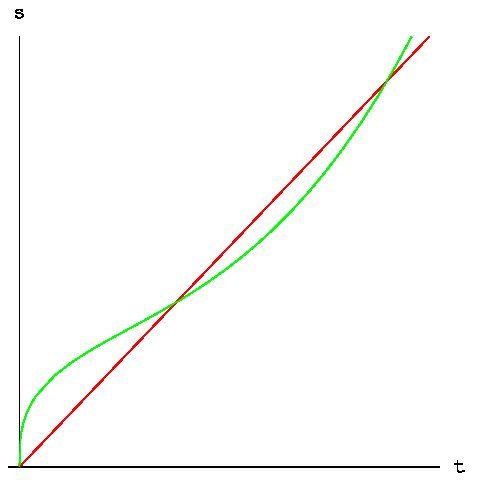 Figure 1
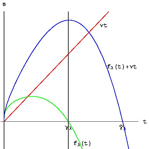 Figure 2
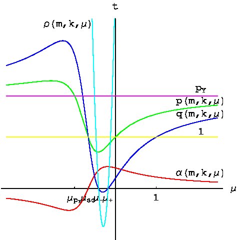 Figure 3
Peer Reviews
No public reviews on file for this paper yet. If you reviewed it on a platform where reviews are public (OpenReview, ICLR, NeurIPS, ICML), you can paste yours below so the community can read it here.
Videos
No videos yet. Explain this paper in a talk, walkthrough, or lecture? Add one.
About Curvature, Conformal Metrics and Warped Products
Fernando Dobarro
&
Bülent Ünal
Dipartimento di Matematica e Informatica, Università degli Studi di Trieste, Via Valerio 12/b, I-34127 Trieste, Italy
Department of Mathematics, Bilkent University, Bilkent, 06800 Ankara, Turkey
Abstract.
We consider the curvature of a family of warped products of two pseduo-Riemannian manifolds and furnished with metrics of the form and, in particular, of the type , where are smooth functions and is a real parameter. We obtain suitable expressions for the Ricci tensor and scalar curvature of such products that allow us to establish results about the existence of Einstein or constant scalar curvature structures in these categories. If is Riemannian, the latter question involves nonlinear elliptic partial differential equations with concave-convex nonlinearities and singular partial differential equations of the Lichnerowicz-York type among others.
Key words and phrases:
Warped products, conformal metrics, Ricci curvature, scalar curvature, semilinear equations, positive solutions, Lichnerowicz-York equation, concave-convex nonlinearities, Kaluza-Klein theory, string theory
1991 Mathematics Subject Classification:
Primary: 53C21, 53C25, 53C50
Secondary: 35Q75, 53C80, 83E15, 83E30.
1. Introduction
The main concern of this paper is the curvature of a special family of warped pseudo-metrics on product manifolds. We introduce a suitable form for the relations among the involved curvatures in such metrics and apply them to the existence and/or construction of Einstein and constant scalar curvature metrics in this family.
Let and be two pseudo-Riemannian manifolds of dimensions and respectively and also let be the usual product manifold of and . For a given smooth function , the warped product was defined by Bishop and O’Neill in [19] in order to study manifolds of negative curvature.
In this article, we deal with a particular class of warped products, i.e. when the pseudo-metric in the base is affected by a conformal change. Precisely, for given smooth functions we will call as a -base conformal warped product (briefly -bcwp), denoted by . We will concentrate our attention on a special subclass of this structure, namely when there is a relation between the conformal factor and the warping function of the form , where is a real parameter and we will call the -bcwp as a -bcwp. Note that we generically called the latter case as special base conformal warped products, briefly sbcwp in [29].
As we will explain in §2, metrics of this type play a relevant role in several topics of differential geometry and theoretical physics (see also [29]). This article concerns curvature related questions of these metrics which are of interest not only in the applications, but also from the points of view of differential geometry and the type of the involved nonlinear partial differential equations (PDE), such as those with concave-convex nonlinearities and the Lichnerowicz-York equations.
The article is organized in the following way: in §2 after a brief description of several fields where pseudo-metrics described as above are applied, we formulate the curvature problems that we deal within the next sections and give the statements of the main results. In §3, we state Theorems 2.2 and 2.3 in order to express the Ricci tensor and scalar curvature of a -bcwp and sketch their proofs (see [29, Section 3] for detailed computations). In §4 and 5, we establish our main results about the existence of -bcwp’s of constant scalar curvature with compact Riemannian base.
2. Motivations and Main results
As we announced in the introduction, we firstly want to mention some of the major fields of differential geometry and theoretical physics where base conformal warped products are applied.
**i: **
In the construction of a large class of non trivial static anti de Sitter vacuum space-times
- **•: **
In the Schwarzschild solutions of the Einstein equations (see [10, 18, 41, 59, 69, 74]).
- **•: **
In the Riemannian Schwarzschild metric, namely (see [10]).
- **•: **
In the “generalized Riemannian anti de Sitter black hole metrics” (see §3.2 of [10] for details).
- **•: **
In the Bañados-Teitelboim-Zanelli (BTZ) and de Sitter (dS) black holes (see [1, 15, 16, 28, 45] for details).
Indeed, all of them can be generated by an approach of the following type: let be a pseudo-Riemannian manifold and be a pseudo-metric on defined by
[TABLE]
After the change of variables , , there results and . Then (2.1) is equivalent to
[TABLE]
Note that roughly speaking, is a nested application of two -bcwp’s. That is, on and taking
[TABLE]
the metric inside the brackets in the last member of (2.2) is a -bcwp, while the metric on is a -bcwp with
[TABLE]
In the last section of [29], through the application of Theorems 2.2 and 2.3 below and several standard computations, we generalized the latter approach to the case of an Einstein fiber with dimension .
**ii: **
In the study of the equivariant isometric embeddings of space-time slices in Minkowski spaces (see [39, 38]).
**iii: **
In the Kaluza-Klein theory (see [76, §7.6, Particle Physics and Geometry], [60] and [77]) and in the Randall-Sundrum theory [30, 40, 63, 64, 65, 71] with as a free parameter. For example, in [46] the following metric is considered
[TABLE]
with the notation , for the coordinates in the 4-dimensional space-time and for the fifth coordinate on an extra dimension. In particular, Ito takes the ansatz
[TABLE]
which corresponds exactly to our sbcwp metrics, considering , , and .
**iii: **
In String and Supergravity theories, for instance, in the Maldacena conjecture about the duality between compactifications of M/string theory on various Anti-de Sitter space-times and various conformal field theories (see [55, 62]) and in warped compactifications (see [40, 72] and references therein). Besides all of these, there are also frequent occurrences of this type of metrics in string topics (see [33, 34, 35, 36, 37, 53, 61, 71] and also [1, 12, 67] for some reviews about these topics).
**iv: **
In the derivation of effective theories for warped compactification of supergravity and the Hor̆ava-Witten model (see [50, 51]). For instance, in [51] the ansatz is considered where is a four-dimensional space-time with coordinates , is a Calabi-Yau manifold (the so called internal space) and depends on the four-dimensional coordinates , in order to study the dynamics of the four-dimensional effective theory. We note that in those articles, the structure of the expressions of the Ricci tensor and scalar curvature of the involved metrics result particularly useful. We observe that they correspond to very particular cases of the expressions obtained by us in [29], see also Theorems 2.2 and 2.3 and Proposition 2.4 stated below.
**v: **
In the discussion of Birkhoff-type theorems (generally speaking these are the theorems in which the gravitational vacuum solutions admit more symmetry than the inserted metric ansatz, (see [41, page 372] and [17, Chapter 3]) for rigorous statements), especially in Equation 6.1 of [66] where, H-J. Schmidt considers a special form of a bcwp and basically shows that if a bcwp of this form is Einstein, then it admits one Killing vector more than the fiber. In order to achieve that, the author considers for a specific value of , namely , in the following problem:
Does there exist a smooth function such that the corresponding -bcwp is an Einstein manifold? (see also (Pb-Eins.) below.)
**vi: **
In the study of bi-conformal transformations, bi-conformal vector fields and their applications (see [32, Remark in Section 7] and [31, Sections 7 and 8]).
**vii: **
In the study of the spectrum of the Laplace-Beltrami operator for forms. For instance in Equation of [11], the author considers the structure that follows: let be an -dimensional compact, Riemannian manifold with boundary, and let be a boundary-defining function; she endows the interior of with a Riemannian metric such that in a small tubular neighborhood of in , takes the form
[TABLE]
where and is the Riemannian metric on (see [11, 56] and references therein for details).
Notation 2.1*.*
From now on, we will use the Einstein summation convention over repeated indices and consider only connected manifolds. Furthermore, we will denote the Laplace-Beltrami operator on a pseudo-Riemannian manifold by i.e., Note that is elliptic if is Riemannian and it is hyperbolic when is Lorentzian. If is neither Riemannian nor Lorentzian, then the operator is ultra-hyperbolic.
Furthermore, we will consider the Hessian of a function , denoted by or , so that the second covariant differential of is given by . Recall that the Hessian is a symmetric tensor field satisfying
[TABLE]
for any smooth vector fields on
For a given pseudo-Riemannian manifold we will denote its Riemann curvature tensor, Ricci tensor and scalar curvature by , and , respectively.
We will denote the set of all lifts of all vector fields of by Note that the lift of a vector field on denoted by is the vector field on given by where is the usual projection map.
In Section 3, we will sketch the proofs of the following two theorems related to the Ricci tensor and the scalar curvature of a generic -bcwp.
Theorem 2.2**.**
Let and be two pseudo-Riemannian manifolds with and , respectively and also let be a real number with
[TABLE]
Suppose . Then the Ricci curvature tensor of the corresponding -bcwp, denoted by Ric verifies the relation
[TABLE]
where
[TABLE]
Theorem 2.3**.**
Let and be two pseudo-Riemannian manifolds of dimensions and respectively. Suppose that and denote the scalar curvatures of and respectively. If and , then the scalar curvature of the corresponding -bcwp verifies,
- (i)
If , then
[TABLE]
where
[TABLE]
[TABLE]
and .
- (ii)
If , then
[TABLE]
From the mathematical and physical points of view, there are several interesting questions about -bcwp’s. In [29] we began the study of existence and/or construction of Einstein -bcwp’s and those of constant scalar curvature. These questions are closely connected to Theorems 2.2 and 2.3.
In [29], by applying Theorem 2.2, we give suitable conditions that allow us to study some particular cases of the problem:
(Pb-Eins.) Given , does there exist a smooth function such that the corresponding -bcwp is an Einstein manifold?
In particular, we obtain the following result as an immediate corollary of Theorem 2.2.
Proposition 2.4**.**
Let us assume the hypothesis of Theorem 2.2. Then the corresponding -bcwp is an Einstein manifold with if and only if is Einstein with constant and the system that follows is verified
[TABLE]
where the coefficients are given by (2.10).
Compare the system (2.15) with the well known one for a classical warped product in [18, 49, 59]. By studying (2.15), we have obtained the generalization of the construction exposed in the above motivational examples in i and v, among other related results. We suggest the interested reader consider the results about the problem (Pb-Eins.) stated in [29].
Now, we focus on the problems which we will deal in §4. Let and be pseudo-Riemannian manifolds.
There is an extensive number of publications about the well known Yamabe problem namely:
(Ya) [79, 75, 68, 13] Does there exist a function such that has constant scalar curvature?
Analogously, in several articles the following problem has been studied:
(cscwp) [27] Is there a function such that the warped product has constant scalar curvature?
In the sequel we will suppose that is a Riemannian manifold.
Thus, both problems bring to the study of the existence of positive solutions for nonlinear elliptic equations on Riemannian manifolds. The involved nonlinearities are powers with Sobolev critical exponent for the Yamabe problem and sub-linear (linear if the dimension of the fiber is ) for the problem of constant scalar curvature of a warped product.
In Section 4, we deal with a mixed problem between (Ya) and (cscwp) which is already proposed in [29], namely:
(Pb-sc) Given , does there exist a function such that the corresponding -bcwp has constant scalar curvature?
Note that when (Pb-sc) corresponds to the problem (cscwp), whereas when the dimension of the fiber and , then (Pb-sc) corresponds to (Ya) for the base manifold. Finally (Pb-sc) corresponds to (Ya) for the usual product metric with a conformal factor in when .
Under the hypothesis of Theorem 2.3 i, the analysis of the problem (Pb-sc) brings to the study of the existence and multiplicity of solutions of
[TABLE]
where all the components of the equation are like in Theorem 2.3 i and (the conjectured constant scalar curvature of the corresponding -bcwp) is a real parameter. We observe that an easy argument of separation of variables, like in [24, §2] and [27], shows that there exists a positive solution of (2.16) only if the scalar curvature of the fiber is constant. Thus this will be a natural assumption in the study of (Pb-sc).
Furthermore, note that the involved nonlinearities in the right hand side of (2.16) dramatically change with the choice of the parameters, an exhaustive analysis of these changes is the subject matter of [29, §6].
There are several partial results about semi-linear elliptic equations like (2.16) with different boundary conditions, see for instance [2, 5, 6, 9, 21, 23, 26, 73, 78] and references in [29].
In this article we will state our first results about the problem (Pb-sc) when the base is a compact Riemannian manifold of dimension and the fiber has non-positive constant scalar curvature .
For brevity of our study, it will be useful to introduce the following notation: and ( as scalar curvature and as Yamabe). Notice that .
We plan to study the case of in a preceding project, therefore the related results are not going to be presented here.
We can synthesize our results about (Pb-sc) in the case of non-positive as follow.
- •
The case of scalar flat fiber, i.e. .
Theorem 2.5**.**
If the answer to (Pb-sc) is affirmative.
By assuming some additional restrictions on the scalar curvature of the base , we obtain existence results for the range .
- •
The case of fiber with negative constant scalar curvature, i.e. .
In order to describe the ranges of validity of the results, we will apply the notations introduced in [29, §5] (see Appendix A for a brief introduction of these notations).
Theorem 2.6**.**
If “ and ” or “ and ” or “ and ”, then the answer to (Pb-sc) is affirmative.
Remark 2.7*.*
The first two cases in Theorem 2.6 will be studied by adapting the ideas in [5] and the last case by applying the results in [73, p. 99]. In the former - Theorem 4.15, the involved nonlinearities correspond to the so called concave-convex whereas in the latter - Theorem 4.16, they are singular as in the Lichnerowicz-York equation about the constraints for the Einstein equations (see [22], [43], [58], [57, p. 542-543] and [73, Chp.18]).
Similarly to the case of , we obtain existence results for some remaining ranges by assuming some additional restrictions for the scalar curvature of the base .
Naturally the study of (Pb-sc) allows us to obtain partial results of the related question:
Given and does there exist a function such that the corresponding -bcwp has constant scalar curvature ?
These are stated in the several theorems and propositions in §4.
3. The curvature relations - Sketch of the proofs
The proofs of Theorems 2.2 and 2.3 require long and yet standard computations of the Riemann and Ricci tensors and the scalar curvature of a general base conformal warped product. Here, we reproduce the results for the Ricci tensor and the scalar curvature, and we also suggest the reader see [29, §3] for the complete computations.
Theorem 3.1**.**
The Ricci tensor of -bcwp, denoted by satisfies
- (1)
* *
* *
* , * 2. (2)
, 3. (3)
* *
* .*
Theorem 3.2**.**
The scalar curvature of a -bcwp is given by
[TABLE]
The following two lemmas (3.3 and 3.7) play a central role in the proof of Theorems 2.2 and 2.3. Indeed, it is sufficient to apply them in a suitable mode and make use of Theorems 3.1 and 3.2 several times, the reader can find all the details in [29, §2 and 4].
Let be a pseudo-Riemannian manifold of dimension , and .
Lemma 3.3**.**
Let be a differential operator on defined by
[TABLE]
where and , . Then,
- (i)
[TABLE]
- (ii)
If and , for and then we have
[TABLE]
Remark 3.4*.*
We also applied the latter lemma in the study of curvature of multiply warped products (see [28]).
Corollary 3.5**.**
Let be a differential operator defined by
[TABLE]
where and . Then, by changing the variables with , and there results
[TABLE]
Remark 3.6*.*
By the change of variables as in Corollary 3.5 equations of the type
[TABLE]
transform into
[TABLE]
Lemma 3.7**.**
Let be a differential operator on defined by
[TABLE]
* and , where the indices extend from to and any . Hence,*
[TABLE]
where is the usual tensorial product. If furthermore, and , then
[TABLE]
where and .
4. The problem (Pb-sc) - Existence of solutions
Throughout this section, we will assume that B is not only a Riemannian manifold of dimension , but also “compact” and connected. We further assume that is a pseudo-Riemannian manifold of dimension with constant scalar curvature . Moreover, we will assume that .
Hence, we will concentrate our attention on the relations (2.11), (2.12) and (2.13) by applying Theorem 2.3 (i).
Let denote the principal eigenvalue of the operator
[TABLE]
and be the corresponding positive eigenfunction with , where is as in Theorem 2.3.
First of all, we will state some results about uniqueness and non-existence of positive solutions for Equation (2.16) under the latter hypothesis.
About the former, we adapt Lemma 3.3 in [5, p. 525] to our situation (for a detailed proof see [5], [20, Method II, p. 103] and also [70]).
Lemma 4.1**.**
Let such that is decreasing. If and satisfy
[TABLE]
and
[TABLE]
then on .
Proof.
Let be a smooth nondecreasing function such that for and for . Thus for all ,
[TABLE]
is smooth, nondecreasing, nonnegative and for and for . Furthermore satisfies for any .
On the other hand, since is a compact Riemannian manifold without boundary and , like in [5, Lemma 3.3, p. 526] there results
[TABLE]
Hence, by the above considerations about and , (4.4) implies that
[TABLE]
Now, by applying (4.2) and (4.3) there results
[TABLE]
Thus by combining (4.6) and (4.5), as we led to
[TABLE]
and conclude the proof like in [5, Lemma 3.3, p. 526-527]. But on and hence ; thus . 111meas denotes the usual measure on the compact Riemannian manifold ∎
Corollary 4.2**.**
Let such that is decreasing. Then
[TABLE]
has at most one solution.
Proof.
Assume that and are two solutions of (4.8). Then by applying Lemma 4.1 firstly with and , and conversely with and , the conclusion is proved. ∎
Remark 4.3*.*
Notice that Lemma 4.1 and Corollary 4.2 allow the function to be singular at [math].
Related to the non-existence of smooth positive solutions for Equation (2.16), we will state an easy result under the general hypothesis of this section.
Proposition 4.4**.**
*If either or
, then (2.16) has no solution in .*
Proof.
It is sufficient to apply the maximum principle with some easy adjustments to the particular involved coefficients. ∎
The case of scalar flat fiber, i.e. .
In this case, the term containing the nonlinearity becomes non-influent in (2.16), thus (Pb-sc) equivalently results to the study of existence of solutions for the problem:
[TABLE]
where is a real parameter (i.e., it is the searched constant scalar curvature) and .
Remark 4.5*.*
222Along this article we consider the sign function defined by , where is the characteristic function of the set .
Let and be a solution of
[TABLE]
Hence, by the difference of homogeneity between both members of (4.9), it is easy to show that if satisfies , then is a solution of (4.10), where and .
Thus by (4.9), we obtain geometrically: if the parameter is given in a way that and has constant scalar curvature , then for any verifying , there results that is of scalar curvature , where and given as above.
Theorem 4.6**.**
* The scalar curvature of a -bcwp of base and fiber (i.e., a singly warped product ) is a constant if and only if and is a positive multiple of (i.e., for some ).*
Proof.
First of all note that implies . On the other hand, in this case, the problem (4.9) is linear, so it is sufficient to apply the well known results about the principal eigenvalue and its associated eigenfunctions of operators like (4.1) in a suitable setting. ∎
Theorem 4.7**.**
* The scalar curvature of a -bcwp of base and fiber is a constant , only if . Furthermore,*
- (1)
if then there exists such that has constant scalar curvature [math] if and only if . Moreover, such ’s are the positive multiples of , i.e. , . 2. (2)
if then there exists such that has constant scalar curvature if and only if . In this case, the solution is unique. 3. (3)
if then there exists such that has constant scalar curvature when and is close enough to [math].
Proof.
The condition implies that , i.e., the problem (4.9) is sublinear. Thus, to prove the theorem one can use variational arguments as in [24] (alternatively, degree theoretic arguments as in [7] or bifurcation theory as in [27]).
We observe that in order to obtain the positivity of the solutions required in (4.9), one may apply the maximum principle for the case of and the antimaximum principle for the case of .
The uniqueness for is a consequence of Corollary 4.2. ∎
Remark 4.8*.*
In order to consider the next case we introduce the following notation. For a given such that , let
[TABLE]
where
[TABLE]
Now, we consider the following two cases.
**: **
In this case by adapting [42, Theorem 1.3], there exists such that is a solution of (4.10) and .
**: **
For this specific and important value, analogously to [42, §2], we distinguish three subcases along the study of our problem (4.10), in correspondence with the .
**: **
in this case, there exists such that is a solution of (4.10) and .
**: **
here there exists such that is a solution of (4.10) and .
**: **
this is a more difficult case, let be the sharp Euclidean Sobolev constant
[TABLE]
where is the volume of the unit sphere. Thus, if
[TABLE]
then there exists such that is a solution of (4.10) and . Furthermore, the condition
[TABLE]
is sharp by [42], so that this is independent of the underlying manifold and the potential considered.
The equality case in (4.14) is discussed in [44].
This results allow to establish the following two theorems.
Theorem 4.9**.**
* There exists such that the scalar curvature of is a constant if and only if where and is given by (4.11). Furthermore if then the solution is unique.*
Proof.
The conditions imply that , i.e. the problem (4.9) is superlinear but subcritical with respect to the Sobolev immersion theorem (see [29, Remark 5.5]). By recalling that , it is sufficient to prove that follows.
Let be defined as in the case of in Remark 4.8. If is a solution of (4.9), then multiplying (4.9) by and integrating by parts there results
[TABLE]
Thus since , and are all positive.
Conversely, if is a real constant such that , then by Remark 4.5, is a solution of (4.9), where and .
On the other side, if , then is a solution of (4.9).
Since , the uniqueness for is a consequence of Corollary 4.2. ∎
Theorem 4.10**.**
* If there exists such that the scalar curvature of is a constant , then . Furthermore, if verifying and (4.13), then there exists such that the scalar curvature of is . Besides, if is negative, then there exists at most one such that the scalar curvature of is .*
Proof.
The proof is similar to that of Theorem 4.9, but follows from the application of the case of in Remark 4.8. Like above, the uniqueness of is a consequence of Corollary 4.2. ∎
In the next proposition including the supercritical case, we will apply the following result (see also [73, p.99]).
Lemma 4.11**.**
Let be a compact connected Riemannian manifold without boundary of dimension and be the corresponding Laplace-Beltrami operator. Consider the equation of the form
[TABLE]
where . If there exist and such that
[TABLE]
then (4.16) has a solution satisfying .
Proposition 4.12**.**
* If , then for all there exists such that the scalar curvature of is the constant . Furthermore, the solution is unique.*
Proof.
The conditions imply that .
On the other hand, since is compact, by taking
[TABLE]
we obtain that and . Thus (4.17) is verified.
Hence, the proposition is proved by applying Lemma 4.11 on . Notice that can take positive values and eventually gets close enough to due to the condition of , and consequently the corresponding solution results positive.
Again, since and the uniqueness is a consequence of Corollary 4.2. ∎
Proof.
(of Theorem 2.5) This is an immediate consequence of the above results. ∎
The case of a fiber with negative constant scalar curvature, i.e. .
Here, the (Pb-sc) becomes equivalent to the study of the existence for the problem
[TABLE]
where is a real parameter (i.e., the searched constant scalar curvature), , and .
Remark 4.13*.*
Let be a solution of (4.18).
- (i)
If , then . Indeed, multiplying the equation in (4.18) by and integrating by parts there results:
[TABLE]
where and are positive.
- (ii)
If , then .
- (iii)
If (the warped product case), then . These cases have been studied in [27, 24].
- (iv)
If (the Yamabe problem for the usual product with conformal factor in ), there results .
An immediate consequence of Remark 4.13 is the following lemma.
Lemma 4.14**.**
Let and be given like in Theorem 2.3(i). Suppose further that is a compact connected Riemannian manifold and is a pseudo-Riemannian manifold of constant scalar curvature . If and (for instance when on ), then there is no such that the scalar curvature of is .
Theorem 4.15**.**
[29, Rows 6 and 8 in Table 4]** Under the hypothesis of Theorem 2.3(i), let be a compact connected Riemannian manifold and be a pseudo-Riemannian manifold of constant scalar curvature . Suppose that “ and ” or “ and ”.
- (1)
If , then is the scalar curvature of a if and only if . 2. (2)
*If , then there exists such that is the scalar curvature of a if and only if . *
Furthermore if , then there exists at most one such that has scalar curvature .
Proof.
The proof of this theorem is the subject matter of §5. ∎
Once again we make use of Lemma 4.11 for the next theorem about the singular case and the following propositions.
Theorem 4.16**.**
[29, Row 7 Table 4]** Under the hypothesis of Theorem 2.3(i), let be a compact connected Riemannian manifold and be a pseudo-Riemannian manifold of constant scalar curvature . Suppose that “ and ”, then for any there exists such that the scalar curvature of is . Furthermore the solution is unique.
Proof.
First of all note that the conditions “ and ” imply that and , i.e. the problem (4.18) is superlinear in but singular in .
On the other hand, since is compact, taking
[TABLE]
there result and . Thus (4.17) is verified.
Thus by an application of Lemma 4.11 for we conclude the proof for the existence part.
The uniqueness part just follows from Corollary 4.2. ∎
Remark 4.17*.*
We observe that the arguments applied in the proof of Theorem 4.16 can be adjusted to the case of a compact connected Riemannian manifold with , and , so that some of the situations included in Theorem 4.15. However, both argumentations are compatible but different.
Proof.
(of Theorem 2.6) This is an immediate consequence of the above results. ∎
The approach in the next propositions is similar to Proposition 4.12 and Theorem 4.16.
Proposition 4.18**.**
[29*, Row 10 Table 4]** Let . If , then for all there exists such that the scalar curvature of is the constant . *
Proof.
The condition implies that .
On the other hand, since is compact, taking
[TABLE]
there result and . Thus (4.17) is satisfied.
Thus an elementary application of Lemma 4.11 for proves the proposition. ∎
Proposition 4.19**.**
[29*, Rows 2, 4 and 3 in Table 4]** Let either “ and ” or “ and ” or “ and ”. If , then for all there exists a smooth function such that the scalar curvature of is the constant . *
Proof.
If either “ and ” or “ and ”, then .
On the other hand, since is compact, taking
[TABLE]
there result and . Thus (4.17) is verified and again we can apply Lemma 4.11 for .
If “ and ”, then . Considering the limits as above, and . So, an application of Lemma 4.11 concludes the proof. ∎
Remark 4.20*.*
Notice that in Theorems 4.15 and 4.16 we do not assume hypothesis related to the sign of , unlike in Propositions 4.12, 4.18 and 4.19.
Proposition 4.21**.**
[29, Rows 5 and 9 in Table 4]** Let be.
- (1)
If either “* and ” or “”, then for all there exists a smooth function such that the scalar curvature of is the constant . In the second case, is also unique .* 2. (2)
If either “” or “” and furthermore , then there exists a smooth function such that the scalar curvature of is [math].
Proof.
In both cases , so by considering
[TABLE]
the proof of (1) follows as in the latter propositions, while that of (2) is a consequence of the linear theory and the maximum principle. ∎
Remark 4.22*.*
Finally, we observe a particular result about the cases studied in [27]. If , then and . When the dimension of the fiber is , the exponent . So, writing the involved equation as
[TABLE]
and by applying Lemma 4.11 as above, we obtain that if , then there exists a smooth function such that the scalar curvature of is the constant . Furthermore, by Corollary 4.2 such is unique (see [27, 24] and [25]).
5. Proof of the Theorem 4.15
The subject matter of this section is the proof of the Theorem 4.15, so we naturally assume its hypothesis.
Most of the time, we need to specify the dependence of of (4.18), we will do that by writing . Furthermore, we will denote the right hand side of by .
The conditions either “ and ” or “ and ”, imply that . But the type of nonlinearity in the right hand side of changes with the , i.e. it is purely concave for and concave-convex for .
The uniqueness for is again a consequence of Corollary 4.2.
In order to prove the existence of a solution for with , we adapt the approach of sub and upper solutions in [5].
Thus, the proof of Theorem 4.15 will be an immediate consequence of the results that follows.
Lemma 5.1**.**
* has a solution if and only if .*
Proof.
This situation is included in the results of the second case of Theorem 4.7 by replacing with (see [24, Proposition 3.1]). ∎
Lemma 5.2**.**
Let us assume that is non-empty and define
[TABLE]
- (i)
If , then .
- (ii)
If , then there exists finite such that .
Proof.
- (i)
It is sufficient to observe Remark 4.13 i.
- (ii)
Like in [5], let such that
[TABLE]
Thus, if is a solution of , then
[TABLE]
so .
∎
Lemma 5.3**.**
Let
[TABLE]
- (i)
Let . There exist and such that , so we have
[TABLE]
- (ii)
If , then . As a consequence of that, is finite.
- (iii)
If , then for all there exists a solution of the problem .
Proof.
- (i)
For any
[TABLE]
It is easy to see that
[TABLE]
is a minimum point for and
[TABLE]
Hence there exist and such that (5.4) is verified.
- (ii)
Since , by the maximum principle, there exists a solution of
[TABLE]
Then, applying item (i) above with there exists and such that with we have that
[TABLE]
hence is a supersolution of .
On the other hand, since , for all
[TABLE]
Furthermore, note that is nondecreasing when . Hence for any there exists a small enough verifying
[TABLE]
thus is a subsolution of .
Then for any , (taking eventually smaller if necessary), we have that the above constructed couple sub super solution satisfies
[TABLE]
Now, by applying the monotone iteration scheme, we have that
. Furthermore by Lemma 5.2 (ii) there results is finite.
- (iii)
The proof of this item is completely analogous to Lemma 3.2 in [5]. We will rewrite this to be self contained.
Given , let be a solution of with . Then is a supersolution of and for small enough , the subsolution of verifies , then as above has a solution.
∎
Lemma 5.4**.**
For any , there exists such that for any solution of . Furthermore if is nonnegative, then positive zero of can be choose as .
Proof.
Define (recall that is compact). There are two different situations, namely.
- •
: since there exists such that and , there results , where is the strictly positive zero of .
- •
: we consider . Now, our problem is equivalent to
[TABLE]
But here the potential of is non negative and the function has the same behavior of with a positive zero on the right side of the positive zero of . Thus, repeating the argument for the case of , we proved .
∎
Lemma 5.5**.**
Let . Then for all there exists a solution of .
Proof.
We will apply again the monotone iteration scheme. Define (note that is compact).
- •
: Clearly, the strictly positive zero of is a supersolution of
[TABLE]
for all .
On the other hand, for small enough,
[TABLE]
Then is a subsolution of (5.10) for all .
By taking possibly smaller, we also have
[TABLE]
We note that for large enough values of , the nonlinearity on the right hand side of (5.10), namely , is an increasing function on .
Thus applying the monotone iteration scheme we obtain a strictly positive solution of (5.10), and hence a solution of (see [3], [4], [54]).
- •
: In this case, like in Lemma 5.4 we consider . Then, the problem is equivalent to
[TABLE]
where the potential is nonnegative and the function has a similar behavior to with a positive zero on the right side of the positive zero of .
Here, it is clear that is a positive supersolution of
[TABLE]
for all . Hence, we complete the proof similarly to the case of .
∎
Lemma 5.6**.**
Let , , and also let be a positive zero of and be a positive zero of . Then there exists a solution of . Furthermore any solution of satisfies .
Proof.
First of all we observe that if (so ), then is the searched solution of .
Now, we assume that . Since , there results . In this case, one can notice that .
On the other hand, the problem is equivalent to
[TABLE]
By the second part of the proof of Lemma 5.4, if is a solution of (or equivalently (5.15)), then . Besides, since
[TABLE]
and results .
From this point on, the proof of the existence of solutions for (5.15) follows the lines of the second part of Lemma 5.5. ∎
6. Conclusions and future directions
Now, we would like to summarize the content of the paper and to propose our future plans on this topic.
We remark to the reader that several computations and proofs, along with other complementary results mentioned in this article and references can be obtained in [29]. We have chosen this procedure to avoid the involved long computations.
In brief, we introduced and studied curvature properties of a particular family of warped products of two pseudo-Riemannian manifolds which we called as a base conformal warped product. Roughly speaking the metric of such a product is a mixture of a conformal metric on the base and a warped metric. We concentrated our attention on a special subclass of this structure, where there is a specific relation between the conformal factor and the warping function , namely with a real parameter.
As we mentioned in §1 and the first part of §2, these kinds of metrics and considerations about their curvatures are very frequent in different physical areas, for instance theory of general relativity, extra-dimension theories (Kaluza-Klein, Randall-Sundrum), string and super-gravity theories; also in global analysis for example in the study of the spectrum of Laplace-Beltrami operators on -forms, etc.
More precisely, in Theorems 3.1 and 3.2, we obtained the classical relations among the different involved Ricci tensors (respectively, scalar curvatures) for metrics of the form . Then the study of particular families of either scalar or tensorial nonlinear partial differential operators on pseudo-Riemannian manifolds (see Lemmas 3.3 and 3.7) allowed us to find reduced expressions of the Ricci tensor and scalar curvature for metrics as above with , where a real parameter (see Theorems 2.2 and 2.3). The operated reductions can be considered as generalizations of those used by Yamabe in [79] in order to obtain the transformation law of the scalar curvature under a conformal change in the metric and those used in [27] with the aim to obtain a suitable relation among the involved scalar curvatures in a singly warped product (see also [52] for other particular application and our study on multiply warped products in [28]).
In §4 and 5, under the hypothesis that be a “compact” and connected Riemannian manifold of dimension and be a pseudo - Riemannian manifold of dimension with constant scalar curvature , we dealt with the problem (Pb-sc). This question leads us to analyze the existence and uniqueness of solutions for nonlinear elliptic partial differential equations with several kinds of nonlinearities. The type of nonlinearity changes with the value of the real parameter and the sign of . In this article, we concentrated our attention to the cases of constant scalar curvature and accordingly the central results are Theorems 2.5 and 2.6. Although our results are partial so that there are more cases to study in forthcoming works, we obtained also other complementary results under more restricted hypothesis about the sign of the scalar curvature of the base.
Throughout our study, we meet several types of partial differential equations. Among them, most important ones are those with concave-convex nonlinearities and the one so called Lichnerowicz-York equation. About the former, we deal with the existence of solutions and leave the question of multiplicity of solutions to a forthcoming study.
We observe that the previous problems as well as the study of the Einstein equation on base conformal warped products, -bcwp’s and their generalizations to multi-fiber cases, give rise to a reach family of interesting problems in differential geometry and physics (see for instance, the several recent works of R. Argurio, J. P. Gauntlett, M. O. Katanaev, H. Kodama, J. Maldacena, H. -J. Schmidt, A. Strominger, K. Uzawa, P. S. Wesson among many others) and in nonlinear analysis (see the different works of A. Ambrosetti, T. Aubin, I. Choquet-Bruat, J. Escobar, E. Hebey, J. Isenberg, A. Malchiodi, D. Pollack, R. Schoen, S. -T. Yau among others).
Appendix A
Let us assume the hypothesis of Theorem 2.3 (i), the dimensions of the base and of the fiber . In order to describe the classification of the type of nonlinearities involved in (2.11), we will introduce some notation (for a complete study of these nonlinearities see [29, Section 5]). The example in Figure 1 will help the reader to clarify the notation.
Note that the denominator in (2.12) is
[TABLE]
and verifies . Thus in (2.12) is positive if and only if and by the hypothesis in Theorem 2.3 (i), results .
We now introduce the following notation:
[TABLE]
where is defined by (2.12).
Thus, for all given as above, is positive. Indeed, by (A.1), if and only if , where
[TABLE]
But and , so
Unlike , changes sign depending on and . Furthermore, it is important to determine the position of and with respect to as a function of and . In order to do that, we define
[TABLE]
where and
[TABLE]
Note that by (A.1), if and only if . Furthermore if and only if . But here changes its sign as a function of and .
We adopt here the notation in [29, Table 4] below, namely if and if . Thus, if , let and two roots (eventually one, see [29, Remark 5.3]) of , . Besides, if , then ; whereas can take any sign.
The reference list from the paper itself. Each links out to its DOI / PubMed record.
- 1[1] O. Aharony, S. S. Gubser, J. Maldacena, H. Ooguri and Y. Oz, Large N Field Theories, String Theory and Gravity , Physics Reports 323 (2000), 183-386 [ar Xiv:hep-th/9905111].
- 2[2] S. Alama, Semilinear elliptic equations with sublinear indefinite nonlinearities , Advances in Differential Equations 4 No. 6 (1999), 813-842.
- 3[3] H. Amann, On the number of solutions of nonlinear equations in ordered Banach spaces , J. Func. Anal. 11 (1972), 346-384.
- 4[4] H. Amann, Fixed point equations and nonlinear eigenvalue problems in ordered Banach spaces , SIAM Rev. 18 (1976), 620-709.
- 5[5] A. Ambrosetti, N. Brezis and G. Cerami, Combined effects of concave and convex nonlinearities in some elliptic problems , J. Funct. Anal. 122 No. 2 (1994), 519-543.
- 6[6] A. Ambrosetti, J. Garcia Azorero and I. Peral, Existence and multiplicity results for some nonlinear elliptic equations: a survey , Rendiconti di Matematica Serie VII Volume 20 (2000), 167-198.
- 7[7] A. Ambrosetti and P. Hess, Positive solutions of asymptotically linear elliptic eigenvalue problems , J. Math. Anal. Appl. 73 (1980), 411-422.
- 8[8] A. Ambrosetti, A. Malchiodi and W-M.Ni, Singularly Perturbed Elliptic Equations with Symmetry: Existence of Solutions Concentrating on Spheres, Part I , (2002).