Yield Curve Shapes and the Asymptotic Short Rate Distribution in Affine One-Factor Models
Martin Keller-Ressel, Thomas Steiner

TL;DR
This paper analyzes the shapes of yield curves and the long-term distribution of the short rate in one-factor affine interest rate models, providing conditions for convergence and characterizing the limit distribution.
Contribution
It characterizes all possible yield curve shapes and describes the asymptotic distribution of the short rate in affine models, including jump-diffusion variants.
Findings
Yield curves are only normal, inverse, or humped.
Conditions for short rate convergence to a limit distribution.
Explicit description of the limit distribution in affine models.
Abstract
We consider a model for interest rates, where the short rate is given by a time-homogenous, one-dimensional affine process in the sense of Duffie, Filipovic and Schachermayer. We show that in such a model yield curves can only be normal, inverse or humped (i.e. endowed with a single local maximum). Each case can be characterized by simple conditions on the present short rate. We give conditions under which the short rate process will converge to a limit distribution and describe the limit distribution in terms of its cumulant generating function. We apply our results to the Vasicek model, the CIR model, a CIR model with added jumps and a model of Ornstein-Uhlenbeck type.
Click any figure to enlarge with its caption.
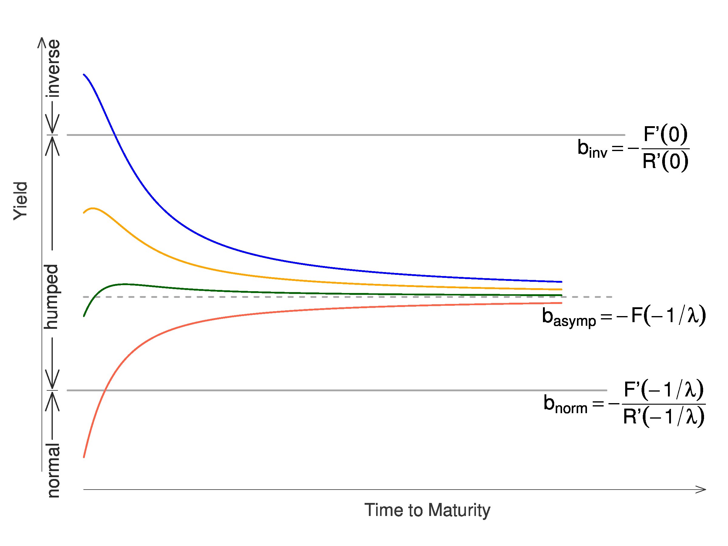 Figure 1
Peer Reviews
No public reviews on file for this paper yet. If you reviewed it on a platform where reviews are public (OpenReview, ICLR, NeurIPS, ICML), you can paste yours below so the community can read it here.
Videos
No videos yet. Explain this paper in a talk, walkthrough, or lecture? Add one.
Taxonomy
TopicsStochastic processes and financial applications · Probability and Risk Models · Financial Risk and Volatility Modeling
Yield Curve Shapes and the Asymptotic Short Rate Distribution in Affine One-Factor Models
Martin Keller-Ressel
Vienna University of Technology, Wiedner Hauptstrasse 8–10, A-1040 Wien, Austria
and
Thomas Steiner
Vienna University of Technology, Wiedner Hauptstrasse 8–10, A-1040 Wien, Austria
Abstract.
We consider a model for interest rates, where the short rate is given under the risk-neutral measure by a time-homogenous, one-dimensional affine process in the sense of Duffie, Filipović, and Schachermayer. We show that in such a model yield curves can only be normal, inverse or humped (i.e. endowed with a single local maximum). Each case can be characterized by simple conditions on the present short rate . We give conditions under which the short rate process will converge to a limit distribution and describe the risk-neutral limit distribution in terms of its cumulant generating function. We apply our results to the Vasiček model, the CIR model, a CIR model with added jumps and a model of Ornstein-Uhlenbeck type.
Key words and phrases:
affine process, term structure of interest rates, Ornstein-Uhlenbeck process, yield curve
Key words and phrases:
affine process, term structure of interest rates, Ornstein-Uhlenbeck process, yield curve
2000 Mathematics Subject Classification:
60J25, 91B28
Supported by the Austrian Science Fund (FWF) through project P18022 and the START programm Y328.
Supported by the module M5 “Modelling of Fixed Income Markets” of the PRisMa Lab, financed by Bank Austria and the Republic of Austria through the Christian Doppler Research Association.
Both authors would like to thank Josef Teichmann for most valuable discussions and encouragement. We also thank various proof-readers at FAM for their comments.
1. Introduction
We consider a model for the term structure of interest rates, where the short rate is given under the martingale measure by a one-dimensional conservative affine process in the sense of Duffie, Filipović, and Schachermayer (2003). An affine short rate process of this type will lead to an exponentially-affine structure of zero-coupon bond prices and thus also to an affine term structure of yields and forward rates.
We emphasize here that the definition of Duffie et al. (2003) is not limited to diffusions, but also includes processes with jumps and even with jumps whose intensity depends in an affine way on the state of the process itself. The class of models we consider naturally includes the Vasiček model, the CIR model and variants of them that are obtained by adding jumps, such as the JCIR-model of Brigo and Mercurio (2006, Section 22.8). Since they are the best-known, the two ‘classical’ models of Vasiček and Cox-Ingersoll-Ross will serve as the starting point for our discussion of yield curve shapes:
A common criticism of the (time-homogenous) CIR and the Vasiček model is that they are not flexible enough to accommodate more complex shapes of yield curves, such as curves with a dip (a local minimum), curves with a dip and a hump, or other shapes that are frequently observed in the markets. Often these shortcomings are explained by ‘too few parameters’ in the model (cf. Carmona and Tehranchi (2006, Section 2.3.5) or Brigo and Mercurio (2006, Section 3.2)). However if jumps are added to the mentioned models, additional parameters (potentially infinitely many) are introduced through the jump part, while the model still remains in the scope of affine models. It is not clear per se what consequences the introduction of jumps will have for the range of attainable yield curves, and this is one question we intend to answer in this article.
Moreover, there seems to be some confusion about what shapes of yield curves are actually attainable even in well-studied models like the CIR-model. While most sources (including the original paper of Cox et al. (1985)) mention inverse, normal and humped shapes, Carmona and Tehranchi (2006, Section 2.3.5) write that ‘tweaking the parameters [of the CIR model] can produce yield curves with one hump or one dip’, and Brigo and Mercurio (2006, Section 3.2) state that ‘some typical shapes, like that of an inverted yield curve, may not be reproduced by the [CIR or Vasiček] model.’ In our main result, Theorem 3.9, we settle this question and prove that in any time-homogenous, affine one-factor model the attainable yield curves are either inverse, normal or humped. The proof will rely only on tools of elementary analysis and on the characterization of affine processes through the generalized Riccati equations of Duffie et al. (2003).
Another related problem is how the shape of the yield curve is determined by the parameters of the model, and also how – when the parameters are fixed – the yield curve is determined by the level of the current short rate. We show in Section 4.2 that also in this respect the CIR model has not been completely understood and discuss a misconception that originates in (Cox et al., 1985) and is repeated for example in (Rebonato, 1998).
In Section 3.3 we provide conditions under which an affine process converges to a limit distribution. We also characterize the limit distribution in terms of its cumulant generating function, extending results of Jurek and Vervaat (1983) and Sato and Yamazato (1984) for OU-type processes to the class of affine processes. These results can again be interpreted in the context of interest rates, where they can be used to derive the risk-neutral asymptotic distribution of the short rate as goes to infinity.
We conclude our article in Section 4 by applying the theoretical results to several interest rate models, such as the Vasiček model, the CIR model, the JCIR model and an Ornstein-Uhlenbeck-type model.
2. Preliminaries
In this section we collect some key results on affine processes from Duffie et al. (2003). In their article affine processes are defined on the -dimensional state space , and we will try to simplify notation where this is possible in the one-dimensional case. Results on affine processes with state space can also be found in Filipović (2001).
Definition 2.1** (One-dimensional affine process).**
A time-homogenous Markov process with state space or and its semi-group are called affine, if the characteristic function of its transition kernel , given by
[TABLE]
and defined (at least) on
[TABLE]
is exponentially affine in . That is, there exist -valued functions and , defined on , such that
[TABLE]
For subsequent results the following regularity condition for will be needed:
Definition 2.2**.**
An affine process is called regular if it is stochastically continuous and the right hand derivatives
[TABLE]
exist for all and are continuous at .
Definition 2.3**.**
The parameters are called admissible for a process with state space if
[TABLE]
and admissible for a process with state space if
[TABLE]
Moreover define the truncation functions
[TABLE]
and finally the functions , for as
[TABLE]
The next result is a one-dimensional version of the key result of Duffie et al. (2003):
Theorem 2.4** **([Duffie, Filipović, and
Schachermayer](#bib.bib6), Theorem 2.7).
Suppose is a one-dimensional regular affine process. Then it is a Feller process. Let be its infinitesimal generator. Then is a core of , and there exist some admissible parameters such that, for ,
[TABLE]
Moreover and , defined by (2.1), solve the generalized Riccati equations
[TABLE]
Conversely let be some admissible parameters. Then there exists a unique regular affine semigroup with infinitesimal generator (2.4), and (2.1) holds with and given by (2.5).
Closely related to affine processes is the notion of an Ornstein-Uhlenbeck (OU-)type process. These processes are of some importance, since they usually offer good analytic tractability and have been studied for longer than affine processes. Following Sato (1999, Chapter 17) an OU-type process can be defined as the solution of the Langevin SDE
[TABLE]
where is a Lévy process, often called background driving Lévy process (BDLP). In an equivalent definition, an OU-type process is a time-homogenous Markov process, whose transition kernel has the characteristic function
[TABLE]
where is the characteristic exponent of . From the last equation it is immediately seen that every OU-type process is an affine process in the sense of Definition 2.1. It is also seen that in the generalized Riccati equations (2.5) for an OU-type process necessarily . Comparing this with (2.3) and Definition 2.3, it is seen that any regular affine process with state space is a process of OU-type. The reverse, however is not true, as there also exist OU-type processes with state space . We will give an example of such a process in Section 4.4.
Naturally we will not only be interested in the process itself, but also in its integral and in quantities of the type
[TABLE]
where is a bounded function on . The next result is an application of the Feynman-Kac formula for Feller semigroups (cf. Rogers and Williams (1994, Section III.19)) and can be found in Duffie et al. (2003). It relies on the positivity of and is therefore only applicable if .
Proposition 2.5** **([Duffie, Filipović, and
Schachermayer](#bib.bib6), Proposition 11.1).
Let be a one-dimensional, regular affine process with state space . Then the family defined by (2.6) forms a regular, affine semigroup with infinitesimal generator
[TABLE]
We will make extensive use of the convexity and continuous differentiability of the functions and from Definition 2.3. These properties are established in this Lemma:
Lemma 2.6**.**
If then as defined in Definition 2.3 have the following properties:
- (i)
* and .* 2. (ii)
* for all .* 3. (iii)
If on , then is either strictly convex on or for all . The same holds for with replaced by . 4. (iv)
If on , then is continuously differentiable on . Also the one-sided derivatives at and are defined but may take the values (at ) and (at ). The same holds for .
Proof.
Property (i) is obvious. If then by Definition 2.3 such that (ii) follows immediately. If we use the estimate
[TABLE]
for all and , and (ii) follows from (2.3). For Property (iii) note that by the Lévy-Khintchine formula there exists an infinitely divisible random variable , such that is its cumulant generating function, i.e. for . Choosing two distinct numbers , we apply the Cauchy-Schwarz inequality to
[TABLE]
which shows convexity of . The inequality is strict unless there exists some such that almost surely. This can only be the case if is constant a.s., in which case is linear. The same argument applies to . Property (iv) follows from the convexity and from the fact that and are analytic on (cf. Lukacs (1960, Chapter 7)). ∎
3. Theoretical Results
We will now use the theory from the last section to calculate bond prices, yields and other quantities in an interest rate model where the short rate follows a one-dimensional regular affine process under the martingale measure. Naturally we will also make the assumption that is conservative, i.e. that for all . This implies by Duffie et al. (2003, Proposition 9.1) that in Definition 2.3. We will need some additional assumptions which are summarized in the following condition:
Condition 3.1**.**
The one-dimensional affine process is assumed to be regular and conservative. In addition, if the process has state space , such that by Definition 2.3 , we require that
[TABLE]
It will be seen that the condition on is necessary to guarantee existence of bond prices for all maturities in the term structure model. By Sato (1999, Theorem 25.17) we get an equivalent formulation of Condition 3.1, if we replace by . Next we define a quantity that will generalize the coefficient of mean reversion from OU-type processes:
Definition 3.2** (quasi-mean-reversion).**
Given a one-dimensional conservative affine process , define the quasi-mean-reversion as the positive solution of
[TABLE]
If there is no positive solution we set .
Since is by Lemma 2.6 a convex function satisfying , it is easy to see that (3.2) can have at most one solution and thus is well-defined. The name quasi-mean-reversion is derived from the fact that if is a process of OU-type with positive mean-reversion, then and the quasi-mean-reversion is exactly the coefficient of mean reversion of . When the process satisfies Condition 3.1, it is seen that must be defined at least on .
We will encounter several times the condition that . The next result gives an equivalent formulation in terms of :
Proposition 3.3**.**
The quasi-mean reversion is strictly positive if and only if , , or .
Proof.
First note that by Lemma 2.6 for all . Using the estimate (2.7) and a dominated convergence argument it is seen from (2.3) that
[TABLE]
where can also take the value . Suppose now that . Then by (3.3) we get . Since and is continuous it follows that there exists a such that . Similarly if , but , it follows from (3.4) that and thus again that .
Conversely, suppose that and . Then
[TABLE]
By the convexity of it follows that for all . Since this implies that for all , and consequently that . ∎
3.1. Bond Prices
We consider now the price of a zero-coupon bond with time to maturity , at time , given by
[TABLE]
The affine structure of carries over to the bond prices, and we get the following result:
Proposition 3.4**.**
*Let the short rate be given by a one-dimensional affine process satisfying Condition 3.1.
Then the bond price exists for all and is given by*
[TABLE]
where and solve the generalized Riccati equations
[TABLE]
Proof.
If the assertion follows directly from Proposition 2.5 by noting that .
If then, as discussed after Theorem 2.4, is a process of OU-type and has the simple structure . By Sato (1999, (17.2) - (17.3)) we obtain in this case directly that
[TABLE]
with if and when . As a function of , is continuously decreasing from [math] to if , and from [math] to if . It is therefore seen that the integral on the right side of (3.7) is finite for all if and only if satisfies (3.1), as required by Condition 3.1. ∎
Corollary 3.5**.**
Let satisfy Condition 3.1 and have quasi-mean-reversion . Then the function from Proposition 3.4 is strictly decreasing and satisfies
[TABLE]
Proof.
The result follows from a qualitative analysis of the autonomous ODE (3.6b). Let . Since the point is an critical point of (3.6b). By the convexity of and the fact that it follows that such that is asymptotically stable, i.e. solutions entering a small enough neighborhood of must converge to . Since for and there is no other critical point in , we conclude that – the solution of (3.6b) starting at [math] – is strictly decreasing and converges to .
If then there is no critical point in and for . It follows that is strictly decreasing and diverges to . ∎
3.2. The Yield Curve and the Forward Rate Curve
The next results are the central theoretical results of this article and describe the global shapes of attainable yield curves in any affine one-factor term structure model.
Definition 3.6**.**
The (zero-coupon) yield is given by and
[TABLE]
For fixed, we call the function the yield curve.
The (instantaneous) forward rate is given by and
[TABLE]
For fixed, we call the function the forward rate curve.
By l’Hospital’s rule and the generalized Riccati equations (3.6) it is seen that both the yield and the forward rate curve are continuous at [math].
The first quantity associated to the yield curve that we consider, is the asymptotic level of the yield curve as , also known as long-term yield, consol yield or simply ‘long end’.
Theorem 3.7**.**
Let the short rate process be given by a one-dimensional affine process satisfying Condition 3.1 with quasi-mean-reversion .If then
[TABLE]
If then
[TABLE]
Proof.
From (3.6a) we obtain that
[TABLE]
If then by Corollary 3.5
[TABLE]
and the assertion follows by combining (3.8) – (3.11).
If then and
[TABLE]
By setting we obtain the desired result. ∎
From Theorem 3.7 it is clear that for practical purposes only models with will be useful. So far we know that in this case the short end of the yield curve is given by and the long end by . We will now examine what happens between these two endpoints.
Definition 3.8**.**
The yield curve is called
- •
normal if it is a strictly increasing function of ,
- •
inverse if it is a strictly decreasing function of ,
- •
humped if it has exactly one local maximum and no minimum on .
In addition we call the yield curve flat if it is constant over all .
This is our main result on the shapes of yield curves in affine one-factor models:
Theorem 3.9**.**
Let the risk-neutral short rate process be given by a one-dimensional affine process satisfying Condition 3.1 and with quasi-mean-reversion . In addition suppose that and that either or is non-linear. Then the following holds:
- •
The yield curve can only be normal, inverse or humped.
- •
Define
[TABLE]
The yield curve is normal if , humped if and inverse if .
The above theorem is visualized in Figure 1. For its proof we will use a simple Lemma. We state the Lemma without proof, since it follows in an elementary way from the usual definition of a convex function on .
Lemma 3.10**.**
A strictly convex or a strictly concave function on intersects an affine function in at most two points. In the case of two intersection points , the convex function lies strictly below the affine function on the interval ; if the function is concave it lies strictly above the affine function on .
Proof of
Theorem 3.9.
Define the function by
[TABLE]
We will see that the convexity behavior of will be crucial for the shape of the yield curve . From the generalized Riccati equations (3.6) the first derivative of is calculated as
[TABLE]
and the second as
[TABLE]
Note that and are continuously differentiable by Lemma 2.6, and also by (3.6b), such that the second derivative of is well-defined and continuous. Since is strictly decreasing by Corollary 3.5, the factor is positive for all . The sign of therefore equals the sign of
[TABLE]
From the fact that is decreasing and and are convex it is obvious that must be decreasing. We will now show that has at most a single zero in :
- (a)
: We have assumed that either or is non-linear. By Lemma 2.6 this implies that either or is strictly convex, and thus that either or is strictly increasing. If , then it follows that is strictly decreasing and thus has at most a single zero. If , an additional argument is needed: It could happen that is of the form such that and is no longer strictly decreasing. However, by assumption, such that in this case has no zero in . 2. (b)
: In this case, by the admissibility conditions in Definition 2.3, we have necessarily . Also, since either or is non-linear, must be non-linear and thus by Lemma 2.6 strictly convex. It follows that is strictly decreasing and thus has at most a single zero in .
We have shown that is decreasing and has at most a single zero; to determine whether it has a zero for some value of , we consider the two ‘endpoints’ and . First we show that
[TABLE]
Since by Proposition 3.4 it follows that
[TABLE]
We distinguish two cases:
- (a)
If then the assertion (3.16) follows immediately. 2. (b)
Consider the case that : Assume that . Then we have and . This, however, stands in contradiction to our assumption , which implies that (cf. Definition 3.2). Thus we must have and ; in this case it follows that , for all , and we set .
Next we consider the right end of and show that
[TABLE]
Since by Corollary 3.5 we have that
[TABLE]
By assumption , and by Definition 3.2 it holds that . Also , and by the mean value theorem
[TABLE]
for some . Since is increasing, it follows that , and we can deduce (3.17) directly from (3.18).
We summarize our results on the function so far: stays negative on if and positive if . It has a single zero on if and only if . If has a zero on , since is decreasing, the sign of will be positive to the left of the zero and negative to the right of the zero.
Since has the same sign as , the statements above translate in the obvious way to the convexity behavior of . We will now use the convexity behavior of to derive our results about the yield curve.
Consider the equation
[TABLE]
for some fixed . Since this equation has at least one solution, . If then is strictly concave on , and by Lemma 3.10 the equation (3.19) has at most one additional solution . Also, when the solution exists, crosses from above at . Similarly if then is strictly convex, and there exists at most one additional solution to (3.19) on . If the solution exists, then is crossed from below at . In the last case , there exists a – the zero of – such that is strictly convex on and strictly concave on . Now there can exist at most two additional solutions to (3.19) with , such that is crossed from below at and from above at .
Because of definition (3.12), every solution to (3.19), excluding , is also a solution to
[TABLE]
with fixed. Also the properties of crossing from above/below are preserved since is positive. This means that in the case , equation (3.20) has at most a single solution, or in other words, that every horizontal line is crossed by the yield curve at most in a single point. If it is crossed, it is crossed from above. This implies that is a strictly decreasing function of , or following Definition 3.8, that the yield curve is inverse. In the case we have again that (3.20) has at most a single solution and that every horizontal line is crossed from below by the yield curve, if it is crossed. In other words, the yield curve is normal. In the last case of , the yield curve crosses every horizontal line at most twice, in which case it crosses first from below, then from above. Thus in this case the yield curve is humped. ∎
Corollary 3.11**.**
Under the conditions of Theorem 3.9 the instantaneous forward rate curve has the same global behavior as the yield curve, i.e.
[TABLE]
In the second case the maximum of the forward rate curve is , where solves
[TABLE]
Proof.
This follows from the fact that as given in (3.13) is exactly the forward rate . The derivative of the forward rate is therefore , which is given in (3.14) as
[TABLE]
The factor is always positive, and the possible sign changes and zeroes of are discussed in the proof of Theorem 3.9, leading to the stated equivalences. Equation (3.21) is simply the condition . ∎
Corollary 3.12**.**
Under the conditions of Theorem 3.9 it holds that
[TABLE]
whenever the quantities are finite. In addition it holds that
[TABLE]
Remark 3.13*.*
Note that equation (3.23) implies that there is always some such that the yield curve is humped.
Proof.
By the mean value theorem there exists a such that
[TABLE]
Since is convex and thus increasing, it holds that
[TABLE]
Applying the mean value theorem to , there exists another such that
[TABLE]
Since is increasing we deduce that . Assuming that also we get
[TABLE]
Since either or is non-linear, one of the functions is strictly convex by Lemma 2.6. Consequently either both inequalities in (3.24) or in (3.25) are strict. Putting them together we get
[TABLE]
proving (3.22) under the assumption that .
If then by definition . Equation (3.24) still holds, but in (3.25) only the left inequality sign remains valid. Together this still proves that and we have shown (3.22).
To prove (3.23) we distinguish two cases:
- (a)
. In this case it is sufficient to prove and . Consider first . If then by definition and nothing is to prove. If then . By convexity and the assertion follows. Consider now . From (3.25) we know that . By convexity and it follows that . 2. (b)
. In this case it is sufficient to prove and to apply (3.22). As above we have that and that . By Definition 2.3
[TABLE]
with . It follows that , proving the assertion. ∎
The last Corollary of this section shows the interesting fact that the occurrence of a humped yield curve is a necessary and sufficient sign of randomness in the short rate model:
Corollary 3.14**.**
Let the risk-neutral short rate process be given by a one-dimensional affine process satisfying Condition 3.1 with and quasi-mean-reversion . Then the following statements are equivalent:
- (i)
There exists a such that is flat. 2. (ii)
There exists no such that is humped. 3. (iii)
The short rate process is deterministic. 4. (iv)
* and .*
Proof.
Theorem 3.9, together with Corollary 3.12, shows already that implies and . Also, from the form of the generator in (2.4), it is seen that and are equivalent. It remains to show that implies and . Proceeding as in the proof of Theorem 3.9 we obtain instead of (3.15) simply
[TABLE]
The yield curve will be humped if and only if has a single (isolated) zero in . Since is a constant function, this cannot be the case for any and we have shown . By the same arguments as in the proof of Theorem 3.9 the yield curve is flat if and only if is constant and equal to [math]. This is the case if . It remains to show that . Note that . In particular , such that for we are already done. If we have by the admissibility conditions in Definition 2.3 that . Thus and we have shown . ∎
3.3. The Limit Distribution of an Affine
Process
It is well-known that the Gaussian Ornstein-Uhlenbeck process, for example, converges in law to a limit distribution and that this distribution is Gaussian. The goal of this section is to establish a corresponding result for affine processes. While calculating the marginal distributions of an affine process involves solving the generalized Riccati equations (2.5), it will be seen that the limit distribution is much easier obtained and can be determined directly from the functions and .
In the interest rate model considered in the preceding section, the short rate follows an affine process under the martingale measure, such that the results will allow us to characterize the risk-neutral asymptotic short rate distribution. Often also the limit distribution under the objective measure is of interest, but the affine property is in general not preserved by an equivalent change of measure, such that the results are not directly applicable. Nevertheless, for the sake of tractability, conditions on the measure change can be imposed, such that the model is affine under both the objective and the risk-neutral measure. (See Nicolato and Venardos (2003) for an example from option pricing and Cheridito et al. (2005) for more general results). In such a setting the results can also be applied under the objective measure.
Before we state the result, we want to recall that a real-valued random variable is called self-decomposable if for every there exists a random variable , independent of , such that
[TABLE]
Since self-decomposability is a distributional property, we will identify and its law, and refer to both as self-decomposable.
For OU-type processes, limit distributions have been studied for some time; the first results can be found in Jurek and Vervaat (1983) and Sato and Yamazato (1984). The next theorem summarizes these results, and can be found in similar form in Sato (1999, Theorem 17.5):
Theorem 3.15**.**
Let be a OU-type process on . If
[TABLE]
then converges in law to a limit distribution which is independent of and has the following properties:
- (i)
* is self-decomposable.* 2. (ii)
The cumulant generating function satisfies
[TABLE]
Conversely, if is a self-decomposable distribution on and , there exists a unique triplet satisfying the admissibility conditions of Definition 2.3, such that is the limit distribution of the affine process (of OU-type) given by the parameters .
As discussed in Section 2, every regular affine process with state space is of OU-type, such that the above theorem applies. We now state our corresponding result for affine processes on :
Theorem 3.16**.**
Let be a one-dimensional, regular, conservative affine process with state space . If
[TABLE]
then converges in law to a limit distribution which is independent of , and whose cumulant generating function is given by
[TABLE]
Proof.
By Theorem 2.4 the transition kernel of the process has the characteristic function
[TABLE]
where and satisfy the generalized Riccati equations (2.5) for all , and thus in particular for all . Since , [math] is a critical point of the autonomous ODE (2.5b), and by the assumption it is asymptotically stable. By the convexity of , also implies that for all , such that is a strictly increasing function in for all . Since [math] is the only critical point of (2.5b) on it also follows that
[TABLE]
Consequently,
[TABLE]
where the last two equalities follow from (2.5) and the transformation . We will now show that the last integral in (3.28) converges absolutely for all : Since and for all we obtain
[TABLE]
where the inequality follows from the fact that the convex function is supported by its tangent at [math]. From the definition of in (2.2) it is clear that the convergence of the last integral will depend only on the jump part of , i.e. the integral converges if and only if
[TABLE]
Define . For a fixed , it is easily verified that as , and that as . Since the Lévy measure integrates by Definition 2.3, and by assumption, it must also integrate . Applying Fubini’s theorem, (3.29) follows, such that converges for all . In particular , such that the limit in (3.28) is a function that is left-continuous at [math]. By standard results on Laplace transforms of probability measures (cf. Steutel and van Harn (2004, Theorem A.3.1)), the pointwise convergence of cumulant generating functions to a function that is left-continuous at [math] implies convergence in distribution of to a limit distribution with cumulant generating function given by (3.28). ∎
Since the marginal distributions of an affine process are infinitely divisible, also the limit distribution must be infinitely divisible, if it exists. In Theorem 3.15 a stronger result is given for an affine process on : In this case is also self-decomposable. An obvious question is, if this result can be extended to the state space . We will see that the answer is negative. In Section 4.3 an example of an affine process with state space is given, which converges to an infinitely divisible limit distribution that is not self-decomposable. This result is interesting, since it leaves open the possibility of some unexpected properties of the limit distribution of an affine process. For example a self-decomposable distribution is always unimodal, whereas an infinitely divisible distribution might be not.
4. Applications
4.1. The Vasiček model
We apply the results of the last section to the classical Vasiček model
[TABLE]
where is a standard Brownian motion under the risk-neutral measure and . The Vasiček model is arguably the simplest affine model, and no surprises are to be expected here. In fact all results that we state here can already be found in the original paper of Vasiček (1977). We advise the reader to view this paragraph as a warm-up for the following examples.
Clearly is a conservative affine process with
[TABLE]
From the quadratic term in and Definition 2.3, it is seen that has state space . This property is often criticized, since it allows the short rate to become negative.
From Theorem 3.9 we calculate
[TABLE]
such that the yield curve in the Vasiček model is normal if , inverse if and humped in the remaining cases.
The long term yield is calculated from (3.7) as
[TABLE]
in this case exactly the arithmetic mean of and .
Theorem 3.15 applies and the cumulant generating function of the risk-neutral limit distribution satisfies
[TABLE]
for . Hence, is Gaussian with mean and variance .
4.2. The Cox-Ingersoll-Ross model
The Cox-Ingersoll-Ross (CIR)-model was introduced by Cox et al. (1985). In this model the short rate process is given by the SDE
[TABLE]
where is a standard Brownian Motion under the risk-neutral measure and . The process is a conservative affine process with
[TABLE]
From Definition 2.3 it is seen that has state space . The fact that interest rates stay non-negative in the CIR-model is often cited as an advantage of the model over the Vasiček model. Calculating the quasi-mean-reversion (see Definition 3.2), we find that
[TABLE]
From Theorem 3.7 we find that the long-term yield is given by
[TABLE]
The boundary between humped and inverse behavior is calculated from Theorem 3.9 as
[TABLE]
Both quantities and can also be found in (Cox et al., 1985, Eq. (26) and following paragraph). Before we consider , we quote (with notation adapted to (4.4)) from page 394 of (Cox et al., 1985) where the shape of the yield curve is discussed:
‘When the spot rate is below the long-term yield , the term structure is uniformly rising. With an interest rate in excess of , the term structure is falling. For intermediate values of the interest rate, the yield curve is humped.’
In our terminology, they claim that the yield curve is normal for , humped for and inverse for . This stands in clear contradiction to Theorem 3.9 and Corollary 3.12 where we have obtained that yield curves are normal if and only if and that , or – in plain words – that there are yield curves starting strictly below the long-term yield that are still humped.
The claims of Cox et al. (1985) are repeated in (Rebonato, 1998, p. 244f), where even several plots of ‘yield surfaces’ (the yield as a function of and ) are presented as evidence. However Rebonato fails to indicate the level of in the plots, such that the conclusion remains ambiguous.
To clarify the scope of humped yield curves in the CIR-model we calculate from Theorem 3.9:
[TABLE]
The relation is immediately confirmed by noting that is the harmonic mean of and . For a graphical illustration we refer to the second yield curve from below in Figure 1. The plot actually shows CIR yield curves with parameters
[TABLE]
plotted over a time scale of years. The second curve from below starts at , i.e. below the long-term yield, but is visibly humped.
To calculate the limit distribution of , we apply Theorem 3.16: The cumulant generating function of the limit distribution is given by
[TABLE]
This is the cumulant generating function of a gamma distribution with shape parameter and scale parameter . Again this result can already be found in Cox et al. (1985, p. 392).
4.3. An extension of the CIR model
To illustrate the power of the affine setting, we consider now an extension of the CIR model that is obtained by adding jumps to (4.4). We define the risk-neutral short rate process by
[TABLE]
where is a compound Poisson process with intensity and exponentially distributed jumps of mean . This model has been introduced by Duffie and Gârleanu (2001) as a model for default intensity and is used by Filipović (2001) as a short rate model. It can also be found in Brigo and Mercurio (2006) under the name JCIR model. It is easily calculated that
[TABLE]
Solving the generalized Riccati equations (3.6) for and becomes quite tedious, but the quantities can be calculated from Theorem 3.7 and Theorem 3.9 in a few lines: The quasi-mean reversion stays the same as in the CIR model, since does not change. From
[TABLE]
we derive immediately
[TABLE]
where . Note that by setting the jump intensity to zero, the expressions of the (original) CIR model are recovered.
Next we calculate the limit distribution of the model. Using the abbreviations and we obtain
[TABLE]
as the cumulant generating function of the limit distribution under the martingale measure.
We now take a closer look at the distribution , since this will answer the question raised at the end of Section 3.3: For certain parameters, is an example for a limit distribution of an affine process that is infinitely divisible, but not self-decomposable. We consider the case and define
[TABLE]
By Frullani’s integral formula
[TABLE]
for all . Since is non-negative on , is the density of a Lévy measure and (4.11) is seen to be the Lévy-Khintchine representation for the cumulant generating function of the infinitely divisible distribution . In addition, is self-decomposable if and only if is non-negative and non-increasing on (cf. Sato (1999, Corollary 15.11)).
In the case of given by (4.10), it is easily calculated that has a single maximum at . Thus, if , then , such that is non-increasing on and is self-decomposable. If then is increasing in the interval and the limit distribution is infinitely divisible, but not self-decomposable.
4.4. The gamma model
Instead of analyzing the properties of a known model, we will now follow a different route and construct a model that satisfies some given properties. We want to construct an affine process on that has the same limit distribution as the CIR model (i.e. a gamma distribution), but is a process of OU-type. The second property is equivalent to . Considering Theorem 3.16, we know that if we want to obtain a limit distribution, we need . To keep with the notation of the Vasiček model, we will write where . Now by (3.27) the cumulant generating function of the limit distribution is given by
[TABLE]
Let the limit distribution be a gamma distribution with shape parameter and scale parameter . Then and by (4.12)
[TABLE]
Setting and it is seen that is equal to the last term in (4.8). This means that the driving Lévy process of is of the same kind as the process in (4.7), i.e. is a pure jump OU-type process with exponentially distributed jump heights of mean and with jump intensity .
We interpret the affine process we have constructed as a risk-neutral short rate process. It is clear that the bond prices are of the exponentially-affine form (3.5). From the generalized Riccati equation (3.6b) we obtain
[TABLE]
From equation (3.6a) we calculate
[TABLE]
such that the bond prices are given by
[TABLE]
The global shape of the yield curve is described by the quantities
[TABLE]
and it is seen that for the gamma-OU-process is the geometric average of and .
5. Conclusions
In this article we have given, under very general conditions, a characterization of the yield curve shapes that are attainable in term structure models where the risk-neutral short rate is given by a time-homogenous, one-dimensional affine process. Even though the parameter space for this class of models is infinite-dimensional, the scope of attainable yield curves is very narrow, with only three possible global shapes. In addition we have given conditions under which an affine process converges to a limit distribution, and we have characterized the limit distribution in terms of its cumulant generating function, extending some known results on OU-type processes.
The most obvious question for future research is the extension of these results to multi-factor models. It is evident from numerical results that in two-factor models yield curves with e.g. a dip, or also with a dip and a hump, can be obtained. It would be interesting to see if more complex shapes can also be produced, or if there are similar limitations as in the single-factor case. Also, in the one-factor case the dependence of the yield curve shape on the current short rate is basically described by the intervals and . In the two-factor case the partitioning of the state-space might be more complex, and we expect to see more interesting transitions between yield curve types. Another aspect is, that since affine processes as a general framework become better understood, extensions of classical models e.g. by adding jumps, like in the JCIR model described in Section 4.3, become more feasible and attractive for applications.
The reference list from the paper itself. Each links out to its DOI / PubMed record.
- 1Brigo and Mercurio [2006] Damiano Brigo and Fabio Mercurio. Interest Rate Models - Theory and Practice . Springer Finance. Springer, 2nd edition, 2006.
- 2Carmona and Tehranchi [2006] René Carmona and Michael Tehranchi. Interest Rate Models: An Infinite Dimensional Stochastic Analysis Perspective . Springer Finance. Springer, 2006.
- 3Cheridito et al. [2005] Patrick Cheridito, Damir Filipović, and Marc Yor. Equivalent and absolutely continuous measure changes for jump-diffusion processes. The Annals of Applied Probability , 15(3), 2005.
- 4Cox et al. [1985] John C. Cox, Jonathan E. Ingersoll, and Stephen A. Ross. A theory on the term structure of interest rates. Econometrica , 53(2):385–407, 1985.
- 5Duffie and Gârleanu [2001] Darrell Duffie and Nicolae Gârleanu. Risk and valuation of collateralized debt obligations. Financial Analysts Journal , 57(1):41 – 59, 2001.
- 6Duffie et al. [2003] Darrell Duffie, Damir Filipović, and Walter Schachermayer. Affine processes and applications in finance. The Annals of Applied Probability , 13(3):984–1053, 2003.
- 7Filipović [2001] Damir Filipović. A general characterization of one factor affine term structure models. Finance and Stochastics , 5:389–412, 2001.
- 8Jurek and Vervaat [1983] Zbigniew J. Jurek and Wim Vervaat. An integral representation for self-decomposable Banach space valued random variables. Zeitschrift für Wahrscheinlichkeitstheorie und verwandte Gebiete , 62:247–262, 1983.