Environmental noise reduction for holonomic quantum gates
Daniele Parodi, Maura Sassetti, Paolo Solinas, Nino Zangh\`i

TL;DR
This paper investigates how to improve the fidelity of holonomic quantum gates affected by environmental noise by optimizing control parameters, revealing that performance can increase over time and comparing with STIRAP gates.
Contribution
It demonstrates a method to enhance holonomic gate performance through parameter loop optimization and compares their robustness with STIRAP gates.
Findings
Gate fidelity improves over time with proper control choices
Optimized loops in control parameters enhance noise resilience
Holonomic gates can outperform STIRAP under certain conditions
Abstract
We study the performance of holonomic quantum gates, driven by lasers, under the effect of a dissipative environment modeled as a thermal bath of oscillators. We show how to enhance the performance of the gates by suitable choice of the loop in the manifold of the controllable parameters of the laser. For a simplified, albeit realistic model, we find the surprising result that for a long time evolution the performance of the gate (properly estimated in terms of average fidelity) increases. On the basis of this result, we compare holonomic gates with the so-called stimulated Raman adiabatic passage (STIRAP) gates.
Click any figure to enlarge with its caption.
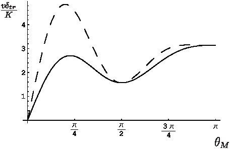 Figure 1
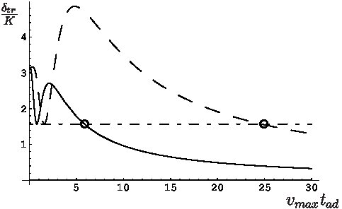 Figure 2
Peer Reviews
No public reviews on file for this paper yet. If you reviewed it on a platform where reviews are public (OpenReview, ICLR, NeurIPS, ICML), you can paste yours below so the community can read it here.
Videos
No videos yet. Explain this paper in a talk, walkthrough, or lecture? Add one.
Environmental noise reduction for holonomic quantum gates
Daniele Parodi,1,2 Maura Sassetti,1,3 Paolo Solinas,4 and Nino Zanghì1,2
1 Dipartimento di Fisica, Università di Genova, Genova, Italy
2 Istituto Nazionale di Fisica Nucleare (Sezione di Genova), Genova, Italy 3 INFM-CNR Lamia
Via Dodecaneso 33, 16146 Genova, Italy
4 Laboratoire de Physique Théorique de la Matière Condensée, Université Pierre et Marie Curie, Place Jussieu, 75252 Paris Cedex 05, France
Abstract
We study the performance of holonomic quantum gates, driven by lasers, under the effect of a dissipative environment modeled as a thermal bath of oscillators. We show how to enhance the performance of the gates by suitable choice of the loop in the manifold of the controllable parameters of the laser. For a simplified, albeit realistic model, we find the surprising result that for a long time evolution the performance of the gate (properly estimated in terms of average fidelity) increases. On the basis of this result, we compare holonomic gates with the so-called Stimulated Raman adiabatic passage (STIRAP) gates.
pacs:
03.67.Lx
I Introduction
The major challenge for quantum computation is posed by the fact that generically quantum states are very delicate objects quite difficult to control with the required accuracy—typically, by means of external driving fields, e.g., a laser. The interaction with the many degrees of freedom of the environment causes decoherence; moreover, errors in processing the information may lead to a wrong output state.
Among the approaches aiming at overcoming these difficulties are those for which the quantum gate depends very weakly on the details of the dynamics, in particular, the holonomic quantum computation (HQC) HQC and the so-called Stimulated Raman adiabatic passage (STIRAP) Kis ; troiani-molinari ; roszak . In the latter, the gate operator is obtained acting on the phase difference of the driving lasers during the evolution, while in the former the same goal is achieved by exploiting the non-commutative analogue of the Berry phase collected by a quantum state during a cyclic evolution. Concrete proposals have been put forward, for both Abelian Jones ; Falci and non-Abelian holonomies HQC_proposal ; HQC_proposal1 ; HQC_proposal2 ; HQC_proposal3 ; HQC_proposal4 ; paper1-2 . The main advantage of the HQC is the robustness against noise deriving from a imperfect control of the driving fields par_noise ; par_noise1 ; par_noise2 ; par_noise3 ; par_noise4 ; par_noise5 ; florio ; fuentes .
In a recent paper hqc_noise we have shown that the disturbance of the environment on holonomic gates can be suppressed and the performance of the gate optimized for particular environments (purely superohmic thermal bath). In the present paper we consider a different sort of optimization, which is independent of the particular nature of the environment.
By exploiting the full geometrical structure of HQC, we show how the performance of a holonomic gate can be enhanced by a suitable choice of the loop in the manifold of the parameters of the external driving field: by choosing the optimal loop which minimizes the “error” (properly estimated in terms of average fidelity loss). Our result is based on the observation that there are different loops in the parameter manifold producing the same gate and, since decoherence and dissipation crucially depend on the dynamics, it is possible to drive the system over trajectories which are less perturbed by the noise. For a simplified, albeit realistic model, we find the surprising result that the error decreases linearly as the gating time increases. Thus the disturbance of the environment can be drastically reduced. On the basis of this result, we compare holonomic gates with the STIRAP gates.
In Sec. II the model is introduced and the explicit expression of the error is derived. In Sec. III we find the optimal loop, calculate the error, make a comparison with other approaches, and briefly sketch how to treat a different coupling with the environment.
II Model
The physical model is given by three degenerate (or quasidegenerate) states, , , and , optically connected to another state . The system is driven by lasers with different frequencies and polarizations, acting selectively on the degenerate states. This model describes various quantum systems interacting with a laser radiation, ranging from semiconductor quantum dots, such as excitons paper1-2 and spin-degenerate electron states troiani-molinari , to trapped ions HQC_proposal1 or neutral atoms HQC_proposal .
The (approximate) Hamiltonian modeling the effect of the laser on the system is (for simplicity, ) HQC_proposal1 ; paper1-2
[TABLE]
where are the timedependent Rabi frequencies depending on controllable parameters, such as the phase and intensity of the lasers, and is the energy of the degenerate electron states. The Rabi frequencies are modulated within the adiabatic time , (which coincides with the gating time), to produce a loop in the parameter space and thereby realize the periodic condition .
The Hamiltonian (1) has four time dependent eigenstates: two eigenstates , , called bright states, and two eigenstates , , called dark states. The two dark states have degenerate eigenvalue and the two bright states have timedependent energies with dark-bright .
The evolution of the state is generated by
[TABLE]
where is the time-ordered operator. In the adiabatic approximation, the evolution of the state takes place in the degenerate subspace generated by , , and . This approximation allows to separate the dynamic contribution and the geometric contribution from the evolution operator. Expanding in the basis of instantaneous eigenstates of (the bright and dark states), in the adiabatic approximation, we have
[TABLE]
where
[TABLE]
here is the operator with matrix elements . The unitary operator plays the role of timedependent holonomic operator and is the fundamental ingredient for realizing complex geometric transformation whereas is the dynamic contribution.
Consider for a closed loop, i.e., for ,
[TABLE]
If the initial state is a superposition of and , then is still a superposition of the same vectors (in general, with different coefficients)paper1-2 . Thus the space spanned by and can be regarded as the “logical space” on which the “logical operator” acts as a “quantum gate” operator. Note that for , has, in general, also a component along . However, as it is easy to show dark-bright , at any instant , can be expanded in the twodimensional space spanned by the dark states and . It is important to observe that depends only on global geometric features of the path in the parameter manifold and not on the details of the dynamical evolution HQC ; paper1-2 .
To construct a complete set of holonomic quantum gates, it is sufficient to restrict the Rabi frequencies in such a way that the norm of the vector is time independent and the vector lies on a real three dimensional sphere HQC_proposal1 ; paper1-2 . We parametrize the evolution on this sphere as , and with fixed initial (and final) point in , the north pole By straightforward calculation we obtain the analytical expression for in eq. (4), , where is the usual Pauli matrix written in the basis of dark states. Thus, the operator (4) becomes , here . Accordingly, the logical operator (5) is
[TABLE]
where
[TABLE]
is the solid angle spanned on the sphere during the evolution. Note that the are many paths on the sphere which generate the same logical operator , and span the same solid angle .
In a previous work we have studied how interaction with the environment disturbs the logical operator hqc_noise . The goal of the present paper is to analyze whether and how such a disturbance can be minimized for a given . To this end, we model the environment as a thermal bath of harmonic oscillators with linear coupling between system and environment caldeira-leggett . The total Hamiltonian is then
[TABLE]
where is the system interaction operator called, from now on, noise operator.
We now consider the time evolution of the reduced density matrix of the system, determined by the Hamiltonian (8). We rely on the standard methods of the “master equation approach,” with the environment treated in the Born approximation and assumed to be at each time in its own thermal equilibrium state at temperature . This allows to include the effect of the environment in the correlation function ()
[TABLE]
Here the spectral density is
[TABLE]
at the low frequencies regimes, is proportional to , with , i.e., describes a Ohmic environments, typical of baths of conduction electrons, describes a super-Ohmic environment, typical of baths of phonons weiss ; hqc_noise . The asymptotic decay of the real part of defines the characteristic memory time of the environment. Denoting with the time evolution of the reduced density matrix of the system in the interaction picture, e.g., , one has weiss
[TABLE]
Here and stand for and , with the tilde denoting the time evolution in the interaction picture.
In quantum information the quality of a gate is usually evaluated by the fidelity , which measures the closeness between the unperturbed state and the final state,
[TABLE]
where is the initial state, and is the reduced density matrix in the Schrödinger picture starting from the initial condition . The average error is defined as the average fidelity loss, i.e.,
[TABLE]
where denotes averaging with respect to the uniform distribution over the initial state .
The right-handside of Eq. (13) can be computed by the following steps:
(1) solving Eq. (11) in strictly second order approximation; this approximation corresponds to replace with ;
(2) using the adiabatic approximation ;
(3) expanding the scalar product in Eq. (13) with respect to a complete orthonormal basis , , orthogonal to . In this way, one obtains
[TABLE]
where
[TABLE]
Here, are the energy differences associated to the transition , with , , , and .
The interaction between system and environment is expressed by the noise operator in Eq. (8). We shall now make the assumption that in the , , and basis. In this case the transition between degenerate states are forbidden, however the noise breaks their degeneracy, shifting one of them. In spite of its simple form, this is nevertheless a realistic noise operator for physical semiconductor systems roszak .
III Minimizing the error
The problem can be stated in the following way: given the noise operator and the logical operator , find a path on the parameter space (the surface of the sphere, described above) which minimizes the error .
The total error , given by Eq. (14), can be decomposed as
[TABLE]
where the transition error, , is the contribution to the sum of the nondegenerate states () and the pure dephasing error is the contribution of the degenerate states (). Thus
[TABLE]
and
[TABLE]
where
[TABLE]
correspond to the transition rates calculated by standard Fermi golden rules, supposing, as usual, for strongly peaked around . In the following we define for simplicity
[TABLE]
Since we are interested at long time evolution, we start discussing the transition error which dominates in this regime roszak ; alicki .
III.1 Transition rate
As explained in Sec. II, the holonomic paths are closed curves on the surface of the sphere which start from the north pole. It turns out that the curve minimizing can be found among the loops which are composed by a simple sequence of three paths (see the Appendix): evolution along a meridian (), evolution along a parallel () and a final evolution along a meridian to come back to the north pole.
The error in (18), depends on given by Eq. (7), (the maximum angle spanned during the evolution along the meridian), (the angle spanned along the parallel), and angular velocity . We allow which corresponds to cover more than one loop along the parallel. The velocity along the parallel is and that along the meridian is . In the following we assume that is constant, and it cannot exceed the maximal value of , fixed by adiabatic condition .
The parameters , , and are connected by the relation . The error is then
[TABLE]
where
[TABLE]
is the contribution along the meridian and
[TABLE]
is the contribution along the parallel.
In Fig. 1 is plotted for and (corresponding to NOT and Hadamard gate, respectively) as a function of . One can see that has a local minimum for and a global minimum for where the error vanishes. This suggests that the best choice is to take as small as possible.
It is interesting to consider the dependence of also on the evolution time . For simplicity, we set the velocity . In this case, changing (and then ) corresponds to a change in the evolution time. We obtain
[TABLE]
where
[TABLE]
Using these relations, and , given by (21) and (22) become functions of , , and . Note that measures the space covered along the parallel, in fact .
In Fig. 2 we see the behavior of as a function of . The first minimum for both curves corresponds to , then the curves for long decrease asymptotically to zero corresponding to the region in which . In this regime we have which is drastically different from the results obtained with other methods where , (see Refs alicki ; roszak and below Sec. III.3). It should be observed that this surprising results is a merit of holonomic approach which allows to choose the loop in the parameter space, without changing the logical operation as long as it subtends the same solid angle. Observe that small and long mean large value of , i.e., multiple loops around the north pole.
Figure 2 shows that, for a given gate, there is a critical value of which discriminate between the choice of (e.g., for the Hadamard gate and for the NOT gate). For the best choice for the loop is ; For the best choice is the value of determined by eq. (23) and (24).
Note that the region is accessible with physical realistic parameters paper1-2 . For example, if we choose the laser intensity meV and (for which values the nonadiabatic transitions are forbidden), the critical parameter corresponds to the critical time of ps for the Hadamard gate and ps for the NOT gate.
III.2 Pure Dephasing
Until now we have ignored the pure dephasing effect because we have assumed that it is negligible in comparison with the transition error for long evolution time. Now, we check that the pure dephasing error contribution can indeed be neglected. We can write the pure dephasing error using Eq. (17) and splitting to parallel and meridian part as
[TABLE]
and
[TABLE]
where .
To estimate we assume that is longer with respect to the characteristic time of the bath. Remembering that , the pure dephasing error behavior along the parallel part at the temperature is
[TABLE]
while the along meridian is
[TABLE]
Then, we can conclude that the pure dephasing can always be neglected for long time evolution because it decreases faster than the transition error.
III.3 Comparison between HQC and STIRAP
We make a comparison between holonomic quantum computation (HQC) and the STIRAP procedure which is an analogous approach to process quantum information. The STIRAP procedure (Kis ; roszak ) is, in its basic points, very similar to the holonomic information manipulation. The level spectrum, the information encoding, the evolution produced by adiabatic evolving laser are exactly the same. The fundamental difference is that in STIRAP the dynamical evolution is fixed (we must pass through a precise sequence of states) and then the corresponding loop in the parameter space is fixed. In particular, we go from the north pole to the south pole and back to the north pole along meridians. Since the loop, as in our model, is a sequence of meridian-parallel-meridian path, we can calculate the error and make a direct comparison. In this case, the transition error results proportional to and grows linearly in time while for HQC . Therefore, the HQC is fundamentally the favorite for long application times with respect to the STIRAP ones.
Moreover, we can show that the freedom in the choice of the loop allows us to construct HQC which perform better than the best STIRAP gates. In Ref. roszak the minimum error (not depending on the evolution time) for STIRAP was obtained reaching a compromise between the necessity to minimize the transition, pure dephasing error and the constraint of adiabatic evolution. With realistic physical parameters hqc_noise (, meV, eV, , meV meV and for low temperature), the total minimum error in Ref. roszak is . With the same parameters, we still have the possibility to increase the evolution time in order to reduce the environmental error. However, for evolution time ps we obtain a total error for the NOT gate and for the Hadamard gate, respectively. As can be seen, the logical gate performance is greatly increased.
III.4 More general noise
Until now we have discussed the possibility to minimize the environmental error by choosing a particular loop in the parameter sphere but the structure of the error functional clearly depends on the system-environment interaction. Then one might wonder if the same approach can be used for a different noise environment.
For this reason, we now briefly analyze the case of noise matrix in the form . Again, for long evolution we can neglect the contribution of the pure dephasing and focus on the transition error. In this case the interesting part of the error functional takes the form
[TABLE]
Even if the analysis in this case is much more complicated, it can be seen that has an absolute minimum for . The long time behavior is the same () such that the results are qualitatively analogous to the above ones: for small loops (or long evolution at fixed velocity) the holonomic quantum gate presents a decreasing error. Then even in this case it is possible to minimize the environmental error.
IV Conclusions
In summary, we have analyzed the performance of holonomic quantum gates in the presence of environmental noise by focusing on the possibility to have small errors choosing different loops in the parameter manifold. Due to the geometric dependence, we can implement the same logical gate with different loops. Since different loops correspond to different dynamical evolutions, we have used this freedom to construct an evolution through “protected” or “weakly influenced” states leading to good holonomic quantum gates performances. This allows to select (once that the physical parameter are fixed) the best loop which minimizes the environmental effect. (Note that this optimization procedure is rather independent of the details of the simple model we have considered and arguably, it could be extended to more complicated systems without any substantial modification.) We have shown that for long time evolutions the noise decreases as while in the other cases it increases linearly with adiabatic time. We also have shown that the same features can be found with different kinds of noise suggesting the possibility to find a way to minimize the environmental effect in the presence of any noise. These results open a new possibility for implementation of holonomic quantum gates to build quantum computation because they seem robust against both control error and environmental noise.
Acknowledgment
The autors thank E. De Vito for useful discussions. One of the authors (P. S.) acknowledges support from INFN. Financial support by the italian MIUR via PRIN05 and INFN is acknowledged.
Appendix A Minimizing theorem
Let us consider the family composed of the closed curves generated by a sequence of paths along a parallel () alternated with paths along a meridian (). We call a generic curve in this family. For example, the family contains all the closed curves composed by the sequence of path meridian-parallel-meridian while the family contains the curves meridian-parallel-meridian-parallel-meridian.
We argue that the closed curve minimizing the error in Eq. (18) can be found in the family. First, we show that any closed curve in spanning a solid angle on the sphere can be replaced by a closed curve in spanning the same angle and producing a smaller error. In analogous way any closed curve in can be replaced by a closed curve in with smaller error and so on. By induction we obtain that any closed curve in can be replaced by a curve in spanning the same solid angle but producing smaller error. Since the curve belonging to can approximate any closed curve on the sphere, the best curve can be found in .
The crucial point is to show that any curve in can be replaced by a curve in . Let us consider a generic curve in spanning a solid angle : composed by a segment of a meridian (with going from [math] to ), a parallel (spanning a angle), meridian (with ), a parallel (spanning a angle), and finally a segment to the north pole along a meridian. Let us consider two closed curves and in subtending the same solid angle with, respectively, and as maximum angle spanned during the evolution along the meridian. First we analyze (20) along the meridian. Without losing generality, we can take ; it is clear from Eq. (21) that the value of along the meridian for is smaller that for : . We note from the Eq. (21), suitable extended to , that the two paths along the meridians depends only on and then produce the same error of ,
[TABLE]
The difference between the contribution along the parallel is
[TABLE]
and
[TABLE]
Analysis of the positivity of the quantities given by Eqs. (31) and (32) shows that cannot be at the same time smaller than and . In fact, there are two possibilities: If , from Eq. (30) and (32),
[TABLE]
and the best closed curve is . If , from Eqs. (30) and (31),
[TABLE]
and the best closed curve is .
In the same way it can be shown that any closed curve in can be replaced by a closed curve in with smaller error.
The reference list from the paper itself. Each links out to its DOI / PubMed record.
- 1(1) P. Zanardi and M. Rasetti, Phys. Lett. A 264 , 94 (1999).
- 2(2) Z. Kis and F. Renzoni, Phys. Rev. A 65 , 032318 (2002).
- 3(3) F. Troiani, E. Molinari, and U. Hohenester, Phys. Rev. Lett. 90 , 206802 (2003).
- 4(4) K. Roszak, A. Grodecka, P. Machnikowski, and T. Kuhn, Phys. Rev. B 71 , 195333 (2005).
- 5(5) J. A. Jones, V. Vedral, A. Ekert, and G. Castagnoli, Nature (London) 403 , 869 (2000).
- 6(6) G. Falci, R. Fazio, G. M. Palma, J. Siewert, and V. Vedral, Nature (London) 407 , 355 (2000).
- 7(7) R. G. Unanyan, B.W. Shore, and K. Bergmann, Phys. Rev. A 59 , 2910 (1999).
- 8(8) L.-M. Duan, J.I. Cirac, and P. Zoller, Science 292 , 1695 (2001).