Effect of node deleting on network structure
Ke Deng, Heping Zhao, Dejun Li

TL;DR
This paper investigates how node deletion affects network structure, revealing transitions from scale-free to exponential degree distributions, development of disassortative correlations, and impacts on connectivity and clustering.
Contribution
It introduces a new network growth model incorporating node deletion, providing insights into structural transformations and stability of evolving networks.
Findings
Degree distribution shifts from scale-free to exponential with increased node deletion
Disassortative degree correlation emerges naturally during evolution
Node deletion does not break network connectivity if edge growth is sufficient
Abstract
The ever-increasing knowledge of the structure of various real-world networks has uncovered their complex multi-mechanism-governed evolution processes. Therefore, a better understanding of the structure and evolution of these networked complex systems requires us to describe such processes in a more detailed and realistic manner. In this paper, we introduce a new type of network growth rule which comprises addition and deletion of nodes, and propose an evolving network model to investigate the effect of node deleting on network structure. It is found that, with the introduction of node deleting, network structure is significantly transformed. In particular, degree distribution of the network undergoes a transition from scale-free to exponential forms as the intensity of node deleting increases. At the same time, nontrivial disassortative degree correlation develops spontaneously as a…
Click any figure to enlarge with its caption.
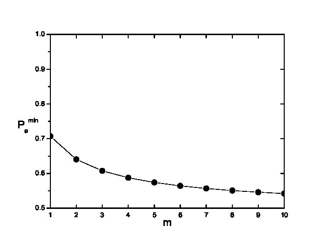 Figure 1
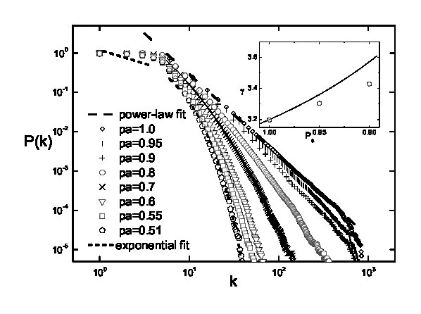 Figure 2
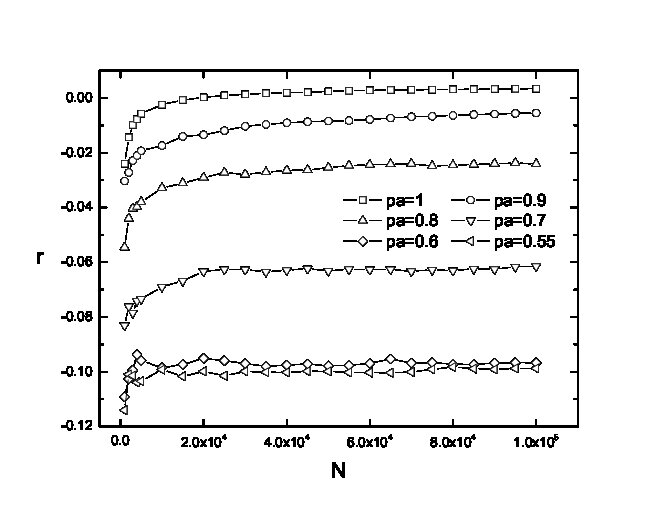 Figure 3
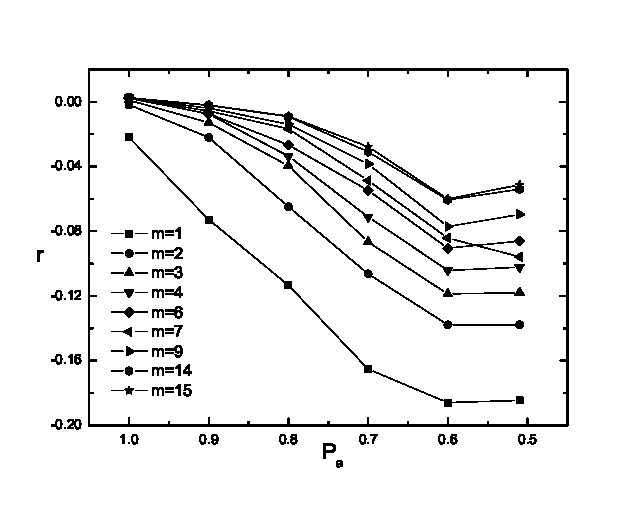 Figure 4
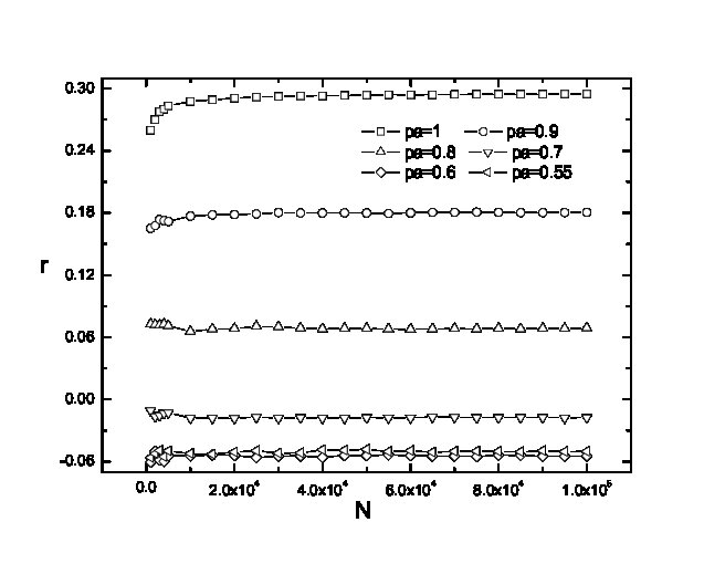 Figure 5
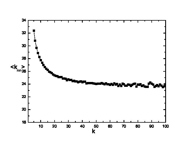 Figure 6
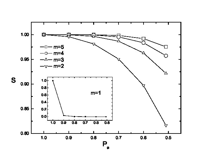 Figure 7
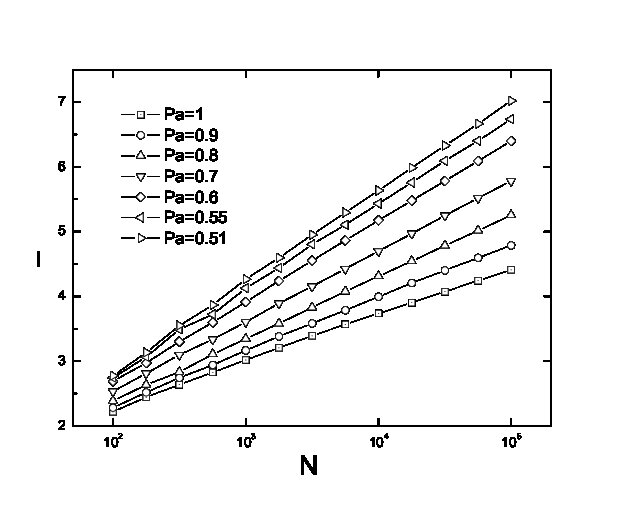 Figure 8
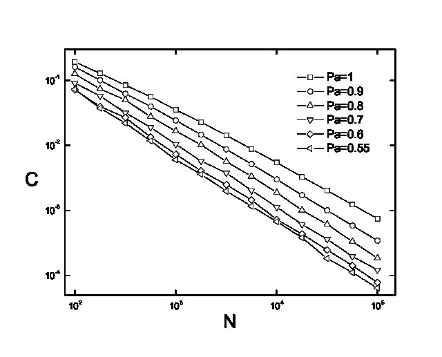 Figure 9
Peer Reviews
No public reviews on file for this paper yet. If you reviewed it on a platform where reviews are public (OpenReview, ICLR, NeurIPS, ICML), you can paste yours below so the community can read it here.
Videos
No videos yet. Explain this paper in a talk, walkthrough, or lecture? Add one.
Effect of node deleting on network structure
Ke Deng
Heping Zhao
Dejun Li
Department of Physics, Jishou University, Jishou, Hunan 416000, People’s Republic of China
Abstract
The ever-increasing knowledge to the structure of various real-world networks has uncovered their complex multi-mechanism-governed evolution processes. Therefore, a better understanding to the structure and evolution of these networked complex systems requires us to describe such processes in more detailed and realistic manner. In this paper, we introduce a new type of network growth rule which comprises of adding and deleting of nodes, and propose an evolving network model to investigate the effect of node deleting on network structure. It is found that, with the introduction of node deleting, network structure is significantly transformed. In particular, degree distribution of the network undergoes a transition from scale-free to exponential forms as the intensity of node deleting increases. At the same time, nontrivial disassortative degree correlation develops spontaneously as a natural result of network evolution in the model. We also demonstrate that node deleting introduced in the model does not destroy the connectedness of a growing network so long as the increasing rate of edges is not excessively small. In addition, it is found that node deleting will weaken but not eliminate the small-world effect of a growing network, and generally it will decrease the clustering coefficient in a network.
I INTRODUCTION
Network structure is of great importance in the topological characterization of complex systems in reality. Actually, these networked complex systems have been found to share some common structural characteristics, such as the small-world properties, the power-law degree distribution, the degree correlation, and so on 1 ; a1 ; 2 . In the theoretical description of these findings, the Watts-Strogatz (WS) model 3 provides a simple way to generate networks with the small-world properties. Barabási and Albert (BA) 4 , with a somewhat different aim, proposed an evolving network model to explain the origin of power-law degree distribution. In this model, by considering two fundamental mechanisms: growth and preferential attachment (PA), power-law degree distribution emerges naturally from network evolution. Based on the framework of BA model, many other mechanisms were introduced into network evolution to reproduce some more complex observed network structures 5 ; 6 ; 7 ; 8 ; 9 ; 10 ; 11 ; 12 ; 13 ; 14 ; a2 ; a5 , such as the degree distribution of broad scale and single scale 5 , as well as the degree correlation a5 . These further studies show that real networked systems may undergo a very complex evolution process governed by multiple mechanisms on which the occurrence of network structures depends. Therefore, to get a better understanding of the structure and evolution of complex networks, describing such processes in more detailed and realistic manner is necessary.
In the BA’s framework, the growing nature of real-world networks is captured by a BA-type growth rule. According to this rule, one node is added into the network at each time step, intending to mimic the growing process of real systems. This rule gives an explicit description to the real-network’ growing process which, however, can in fact be much more complex. One fact is that in many real growing networks, there are constant adding of new elements, but accompanied by permanent removal of old elements (deletion of nodes) 28 ; 15 ; 16 ; 17 ; a3 ; a4 . Take the food webs for a example: there are both additions and losses of nodes (species) at ecological and evolutionary time scales by means of immigration, emigration, speciation, and extinction 28 . Likewise, for Internet and the World Wide Web (WWW), node-deleting is reported experimentally in spit of their rapid expansion of size 15 ; 16 ; 17 ; a3 ; a4 . In the Internet’s Autonomous Systems (ASs) map case, a node is an AS and a link is a relationship between two ASs. An AS adding means a new Internet Service Provider (ISP) or a large institution with multiple stub networks joins the Internet. An AS deleting happens due to the permanent shutdown of the corresponding AS as it is, for example, out of business. Investigations of the evolution of real Internet maps from 1997 to 2000 verified such network mechanism 15 ; 16 ; 17 . The same is for the evolution of WWW, in which the deletions of invalid web pages are also frequently discovered a3 ; a4 . In most cases, the deletion of a node is also accompanied with the removal of all edges once attached to it. These facts justify the investigation of node-deletion’s influence on network structure. In this paper, we introduce a new type of network growth rule which comprises of adding and deleting of nodes, and propose an evolving network model to investigate the effect of node deleting on the network structure. Before now several authors have proposed some models on node removal in networks, such as AJB networks in which a portion nodes are simultaneously removed from the network 18 , and also the decaying 19 and mortal 20 networks, which concerns networks’ scaling property and critical behavior respectively. Sarshar et al 21 investigated the ad hoc network with node removal, focusing on the compensatory process to preserve true scale-free state. They are different from present work, in which node deleting is treated as an ubiquitous mechanism accompanied with the evolution of real-world networks.
This paper is organized as follows. In Section II, an evolving network model taking account of the effect of node deleting is introduced which reduces to a generalized BA model when the effect of node deleting vanishes. Then the effect of node deleting on network structure are investigated in five aspects: degree distribution (Section III), degree correlation (Section IV), size of giant component (Section V), average distance between nodes (Section VI) and clustering (Section VII). Finally, Section VIII presents a brief summary.
II THE MODEL
We consider the following model. In the initial state, the network has isolated nodes. At each time step, either a new node is added into the network with probability or a randomly chosen old node is deleted from the network with probability , where is an adjustable parameter. When a new node is added to the network, it connects to () existing node in the network according to the preferential probability introduced in the BA model 4 , which reads
[TABLE]
where is the degree of node . When an old node is deleted from the network, edges once attached to it are removed as well. In the model, is varied in the range of , since in the case of the network can not grow. In order to give a chance for isolated nodes to receive a new edge, we choose preferential probability proportional to 6 . Note that when , our model reduces to a generalized BA model 22 .
To get a general knowledge to the effect of node deleting on network structure, firstly, a simple analysis to the surviving probability is helpful. Here, is defined as the probability that a node is added into the network at time step , and this node (the th node) has not been deleted until time step , where . Supposing that a node-adding event happens at time step , and the probability that the th node has not been deleted until time step is denoted as . Then, due to the independence of events happened at each time step, it is easy to verify that with , where is the number of nodes in the network at moment (in the limit of large ). In the continuous limit, we obtain
[TABLE]
which yields
[TABLE]
Thus to get the we should multiply with , i.e.
[TABLE]
One can easily find that decreases rapidly as increases and/or as decreases provided . It is well known that highly connected nodes, or hubs, play very important roles in the structural and functional properties of growing networks 1 ; a1 ; 2 . The formation of hubs needs a long time to gain a large number of connections. As a consequence, according to Eq. (4), a large portion of potential hubs are deleted during the network evolution. Thus it can be expected that the introduction of node deleting has nontrivial effects on network structure. In the following we show how network structure can be effected by the node deleting introduced in present model.
III DEGREE DISTRIBUTION
The degree distribution , which gives the probability that a node in the network possesses edges, is a very important quantity to characterize network structure. In fact, has been suggested to be used as the first criteria to classify real-world networks 5 . Therefore it is necessary to investigate the effect of node deleting on the degree distribution of networks firstly. Now we adopt the continuous approach 23 to give a qualitative analysis of for our model with slight node deletion (i.e., when is very small). Supposing that there is a node added into the network at time step , and this node is still in the network at time , let be the degree of the th node at time , where . Then the increasing rate of is
[TABLE]
where
[TABLE]
and the denotes the sum of all during the time step between [math] and . It is easy to verify that the first term in Eq. (5) is the increasing number of links of the th node due to the preferential attachment made by the newly added node. The second term in Eq. (5) accounts for the losing of a link of the th node during the process of node deletion, which happened with the probability .
Firstly we solve for the and get
[TABLE]
(see the Appendix for details). Inserting Eq. (7) back into Eq. (5), one gets
[TABLE]
where
[TABLE]
and
[TABLE]
When , the solution of Eq. (8) is
[TABLE]
Now, to get the probability that a randomly selected node at time will have degree , we need to calculate the expected number of nodes with degree at time . Then the can be obtained from , where is the total number of nodes at time . Let represent the set of all possible nodes with degree at time , then one gets
[TABLE]
In the continuous-time approach, the number of nodes in is the number of ’s for which , and it is approximated to , where is the solution of the equation . To proceed with our analysis, now we make the approximation that all nodes in have the same surviving probability 111It seems that this is not a very good approximation, since investigations indicate that values of are large and increase rapidly with the decrease of . Thus the analysis here is a qualitative one and only suit for the condition of slight node deletion in the model.. Under this mean-field approximation, Eq. (12) can be written as
[TABLE]
From Eq. (11), we obtain
[TABLE]
then
[TABLE]
Inserting Eq. (14) back into Eq. (4) we get
[TABLE]
Inserting Eqs. (15) and (16) into Eq. (13), and noting that , we get
[TABLE]
which is a generalized power-law form with the exponent
[TABLE]
We point out again that equation (11) is only valid when , which translates into , i.e.
[TABLE]
Considering that , Eq. (19) is satisfied when
[TABLE]
In Fig. 1, we plot as a function of . One can see from Fig. 1 that the curve divides our model into two regimes. : in this case and equation (11) is valid. Thus, the degree distribution of the network exhibits a generalized power-law form. : In this case can not be always satisfied and equation (11) is not valid. Therefore, our continuous approach fails to predict the behavior of , and we will investigate it with numerical simulations. The , as one can find from Fig. 1, decreases with the increase of .
In the power-law regime [], the behavior of is predicted by Eqs. (17) and (18), which are obtained using a mean-field approximation [Eq. (13)]. One can easily verify that such approximation is only exact when , in which case Eq. (18) turns into , in good agreement with the results obtained from generalized BA model studied in Ref 22 . If , Eqs. (17) and (18) still give qualitative predictions for the model: with slight node deletion, of the network is still power-law, and the exponential increases with the decrease of (inset of Fig. 2).
In remaining regime [], the limiting case is , in which the growth of network is suppressed (a very slowly growing one). Similar non-growing networks have been studied, for example, for the Model B in Ref24 , and the degree distribution has the exponential form. Here we conjecture that, in this regime, of our model crossovers to an exponential form, which is verified by the numerical simulation results below.
Now we verify the above analysis with numerical simulations. In Fig. 2, we give the cumulative degree distributions 2 of the networks with different . As gradually decreases from to , Fig. 2 shows an interesting transition process which can be roughly divided into three stages. : In this stage, the model works in the power-law regime and the power-law exponent increases as decreases. Inset of Fig. 2 gives the comparison between the value of predicted by Eq. (18) and the one obtained from numerical simulations. One sees that the theory and the simulation results are in perfect agreement for . As decreases, however, the agreement is only qualitative and the deviation between theory and simulation becomes more and more obvious. As we have mentioned above, such increasing deviation is due to the mean-field approximation used in the analysis. These results tell us that slight node deletion does not cause deviation of the network from scale-free state, but only increases its power-law exponent. Such robustness of power-low revealed here gives an explanation to the ubiquity of scale-free networks in reality. It should be noted that a very similar robustness has also been found in the study of network resilience, where simultaneously deleting of a portion of nodes was taken into account in static scale-free networks 18 . : In this stage, the model works in the regime of . As one sees from Fig. 2, of the network behaviors exponentially. This result indicates that with manifest node deletion, the network will deviate from scale-free state and become exponential. : In this stage, a crossover of the model from the power-law regime to the exponential regime is found, in which the is no longer pure scale-free but truncated by an exponential tail. As one can see, the truncation in increases as decreases.
Besides the power-law degree distribution, it is now known that in real world may deviate from a pure power-law form 25 ; 26 ; 27 ; 28 ; 29 . According to the extent of deviation, of real systems has been classified into three groups 5 : scale-free (pure power-law), broad scale (power-law with a truncation), and single scale (exponential). Many mechanisms, such as aging 5 ; 7 ; 8 , cost 5 , and information filtering 9 , have been introduced into network growth to explain these distributions. Here, the results of Fig. 2 indicate that a modified version of growth rule can lead to all the three kinds of in reality, and it provides another explanation for the origin of the diversity of degree distribution in real-world: such diversity may be a natural result of network growth.
IV DEGREE CORRELATION
It has been recently realized that, besides the degree distribution, structure of real networks are also characterized by degree correlations 15 ; 30 ; 31 ; 32 ; 33 . This translates into the fact that degrees at the end of any given edge in real networks are not usually independent, but are correlated with one another, either positively or negatively. A network in which the degrees of adjacent nodes are positively (negatively) correlated is said to show assortative (disassortative) mixing by degree. An interesting observation emerging from the comparing of real networks of different types is that most social networks appear to be assortatively mixed, whereas most technological and biological networks appear to be disassortative. The level of degree correlation can be quantified by the assortativity coefficient lying in the range , which can be written as
[TABLE]
for practical evaluation on an observed network, where , are the degrees of the vertices at the ends of the th edge, with 30 . This formula gives when the corresponding network is positively (negatively) correlated, and when there is no correlation 222Another way to represent degree correlation is to calculate the mean degree of the nearest neighbors of a vertex as a function of the degree of that vertex. Although such way is explicit to characterize degree correlation for highly heterogeneously organized networks, for less heterogeneous networks (this is the case in the proposed model when the intensity of node deleting increases, see Fig. 2), it may be very nosy and difficult to interpret. So here we adopt the assortativity coefficient to characterize degree correlation in the model..
Recently, Maslov et al 34 and Park et al 35 have proposed a possible explanation for the origin of such correlation. They show for a network the restriction that there is at most one edge between any pair of nodes induces negative degree correlations. This restriction seems to be an universal mechanism (indeed, there is no double edges in most real networks), therefore, the authors of Ref. 35 conjecture that disassortativity by degree is the normal state of affairs for a network. Although only a part of the measured correlation can be explained in the way of Ref. 35 , this universal mechanism does give a promising explanation for the origin of degree correlation observed in real networks of various types.
It will be of great interest to discuss the effect of node deleting on degree correlation. In Fig. 3, we give the assortativity coefficient as a function of network size , for different in our model, for . As one sees from Fig. 3, for each value of , after a transitory period with finite-size effect, each of networks tends to reach a steady value. When , as becomes large. This result indicates that networks in the BA model are uncorrelated, in agreement with results obtained in previous studies 30 ; 33 . When , nontrivial negative degree correlations spontaneously develop as networks evolve. One can see from Fig. 3 that the steady value of in the model decreases with the decreasing . In particular, when , the value of is about . These results indicate that node deleting leads to disassortative mixing by degree in evolving networks. To make such relation more clear, in Fig. 4, we plot of networks in our model as a function of , for different . As the Fig. 3 indicates, when the network size is larger than , the assortativity coefficient is nearly stable. So all results in Fig. 4 are obtained from networks with . Fig. 4 gives us the same relation between and shown in Fig. 3. What is more, it tells us that for a given , will increase with the increasing . The increment gets its maximum between and other values. We point out that this is because when , the network has been broke up into small separate components (see the following section). We can also find from Fig. 4 that the gap between different curves decreases with the increasing and the curves tend to merge at large .
Now we give some explanations to the above observations. In the BA model, the network being uncorrelated is the result of a competition between two factors: the growth and the preferential attachment (PA). On the one hand, networks with pure growth is positively correlated. This is because the older nodes, also tending to be higher degree ones, have a higher probability of being connected to one another, since they coexisted earlier. In Fig. 5, we compute the assortativity coefficient of a randomly growing network, which grows by the growth rule of BA-type, while the newly added nodes connect to randomly chosen existing ones. As one can see from Fig. 5 that pure growth leads to positive . On the other hand, the introduction of PA makes the connection between nodes tend to be negatively correlated, since newly added nodes (usually low degree ones) prefer to connect to highly connected ones. Then degree correlation characteristic of the BA model is determined by this two factors. In Fig. 6, we plot the average degree of the nearest neighbor as a function of in the BA model. It is found that nodes with large show no obvious biases in their connections. But there is a short disassortative mixing region when is relatively small (also reported in Ref. a6 , see Fig.1a therein). Such phenomenon can be explained by the effect of these two factor: Growth together with PA makes nodes with large equally connect to both large and small degree nodes, and the latter makes nodes with small degree be disassortatively connected. Now, we introduce node-deletion. According to Eq. (4), depression of the growth of large-degree nodes also decreases the connections between them, therefore makes the correlation negative. We also investigate the effect of node deleting on the of the randomly growing network, and obtained similar results. As one sees from Fig. 5, depression of connections between higher degree nodes causes the network less positively correlated, and with stronger node-deletion, negatively correlated. Finally, with regard to the effect of in this relation (Fig. 4), larger means more edges are established according to the PA probability Eq. (1). We conjecture that the orderliness of newly added nodes connecting to large degree nodes will be weakened by the increasing randomness as becomes larger, thus leading to a less negative correlation. Such randomness can not always increase and, as we see from Fig. 4, for large , e.g., , the curves tend to merge together.
V SIZE OF GIANT COMPONENT
In a network, a set of connected nodes forms a component. If the relative size of the largest component in a network approaches a nonzero value when the network is grown to infinite size, this component is called the giant component of the network 1 ; a1 ; 2 . In most previously studied growing models 1 ; a1 ; 2 , due to the BA-type growth rule they adopted, there is only one huge component in the network, i.e., . In this extreme case the network gains a perfect connectedness. The opposite case of is the extreme of , in which case the network, made up of small components, exhibits no connectedness. Experiments indicate that some real networks seem to lie in somewhere between these two extreme: they contain a giant component as well as many separate components a1 ; 2 ; 36 ; 37 . For example, According to Ref.36 , in May of 1999, the entire WWW, containing pages, consisted of a giant component of pages and the disconnected components (DC) of about pages. In general, the introduction of node deletion in our model will cause the emergence of separate components even isolated nodes in the network. What we interest here is the connectedness of the network. In Fig. 7 we plot the relative size of the largest component in the model, as a function of , for , where is the number of edges generated with the adding of a new node. One sees from Fig. 7 that for any , a giant component can be observed in the model if . In addition, for the same , increase as the increase of . While when , the network is found to be broke up into separate components if . For example, when , of the network with rapidly drops to . Inset of Fig. 7 gives the Vs curve for . These results indicate that node deleting does not destroy the connectedness of a growing network so long as the increasing rate of edges is not excessively small.
VI AVERAGE DISTANCE BETWEEN NODES
Now we study the effect of node deletion on networks’ average distance between nodes. Here the distance between any two nodes is defined as the number of edges along the shortest path connecting them. It has been revealed that, despite their often large size, most real networks present a relatively short , showing the so-called small-world effect 1 ; a1 ; 2 ; 3 . Such an effect has a more precise meaning: networks are said to show the small-world effect if the value of scales logarithmically or slower with network size for fixed mean degree. This logarithmic scaling can be proved for a variety of network models 1 ; a1 ; 2 . As we have demonstrated in Section V, node deleting does not destroy the connectedness of the network in our model for any , since there is always a giant component exists. Here in our simulation, we calculate of the giant component of the network in our model using the burning algorithm 2 . In Fig. 8, we plot as a function of network size , for different in our model. As one can see from the figure, for any , a logarithmic scaling is obtained, while the proportional coefficient increases with the decrease of . Furthermore, for a given , increases with the decrease of . These results tell us that node deleting will weaken but not eliminate the small-world effect of a growing network.
VII CLUSTERING
Finally, we investigate the effect of node deletion on network’s cluster coefficient , which is defined as the average probability that two nodes connected to a same other node are also connected. For a selected node with degree in the network, if there are edges among its nearest neighbors, the cluster coefficient of node is defined as
[TABLE]
Then the clustering coefficient of the whole network is the average of all individual . In Fig. 9, we plot of the giant component in the network as a function of network size , for different . As one sees from Fig. 9, for each , the clustering coefficient of our model decreases with the network size, following approximately a power law form. Such size-dependent property of is shared by many growing network model 1 ; a1 ; 2 . Moreover, as Fig. 9 shows, for the same network-size , decreases as decreases. The results of Fig. 9 indicate that node deleting weakens network’s clustering.
VIII CONCLUSION
In summary, we have introduced a new type of network growth rule which comprises of adding and deleting of nodes, and proposed an evolving network model to investigate effects of node deleting on network structure. It has been found that, with the introduction of node deleting, network structure was significantly transformed. In particular, degree distribution of the network undergoes a transition from scale-free to exponential forms as the intensity of node deleting increased. At the same time, nontrivial disassortative degree correlation spontaneously develops as a natural result of network evolution in the model. We also have demonstrated that node deleting introduced in our model does not destroy the connectedness of a growing network so long as the increasing rate of edge is not excessively small. In addition, it has been observed that node deleting will weaken but not eliminate the small-world effect of a growing network. Finally, we have found that generally node deleting will decrease the clustering coefficient in a network. These nontrivial effects justify further studies of the effect of node deleting on network function 2 , which include topics such as percolation, information and disease transportation, error and attack tolerance, and so on.
Acknowledgements.
The authors thank Doc. Ke Hu for useful discussions. This work is supported by the National Natural Science Foundation of China, Grant No. 10647132, and Natural Science Foundation of Hunan Province, China, Grant No. 00JJY6008.
Appendix A THE CALCULATION OF
To get , we multiply both sides of Eq. (5) by and sum up all between [math] and :
[TABLE]
To get the above equation we have used the definition of [Eq. (6)] and the following equation:
[TABLE]
The left-hand side of Eq. (23) can be simplified as:
[TABLE]
Substituting the above expression in Eq. (23), and noting that and , we get
[TABLE]
The solution to the above equation is
[TABLE]
The reference list from the paper itself. Each links out to its DOI / PubMed record.
- 1(1) R. Albert and A.-L. Barabási, Rev. Mod. Phys. 74 , 47 (2002).
- 2(2) S. N. Dorogovtsev, and J. F. F. Mendes, Adv. Phys. 51 , 1079 (2002).
- 3(3) M. E. J. Newman, SIAM Review 45 , 167 (2003).
- 4(4) D. J. Watts and S.H. Strogatz, Nature (London) 393 , 440 (1998).
- 5(5) A.-L. Barabási and R. Albert, Science, 286 , 509 (1999).
- 6(6) L. A. N. Amaral, A. Scala, M. Barthélémy and H. E. Stanley, Proc. Natl. Acad. Sci. U.S.A. 97 , 11149 (2000).
- 7(7) R. Albert and A.-L. Barabási, Phys. Rev. Lett. 85 , 5234 (2000).
- 8(8) S. N. Dorogovtsev and J. F. F. Mendes, Phys. Rev. E 62 , 1842 (2000).