Spline Single-Index Prediction Model
Li Wang, Lijian Yang

TL;DR
This paper introduces a robust single-index prediction model using spline estimators, effective for high-dimensional, weakly dependent data, with proven consistency, normality, and fast computation, demonstrated through simulations and real data application.
Contribution
It proposes a spline-based single-index prediction method that is robust, computationally efficient, and applicable to high-dimensional, dependent data, extending existing models.
Findings
Spline estimator is root-n consistent and asymptotically normal.
The iterative routine is fast enough for large, high-dimensional data.
Application to Icelandic river flow data shows superior forecasting performance.
Abstract
For the past two decades, single-index model, a special case of projection pursuit regression, has proven to be an efficient way of coping with the high dimensional problem in nonparametric regression. In this paper, based on weakly dependent sample, we investigate the single-index prediction (SIP) model which is robust against deviation from the single-index model. The single-index is identified by the best approximation to the multivariate prediction function of the response variable, regardless of whether the prediction function is a genuine single-index function. A polynomial spline estimator is proposed for the single-index prediction coefficients, and is shown to be root-n consistent and asymptotically normal. An iterative optimization routine is used which is sufficiently fast for the user to analyze large data of high dimension within seconds. Simulation experiments have…
Click any figure to enlarge with its caption.
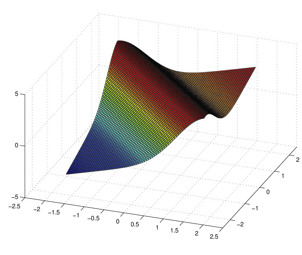 Figure 1
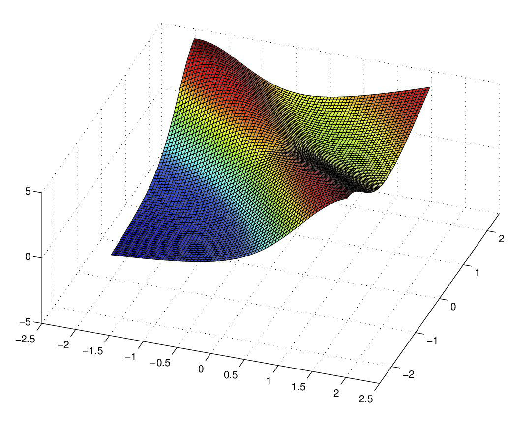 Figure 2
Peer Reviews
No public reviews on file for this paper yet. If you reviewed it on a platform where reviews are public (OpenReview, ICLR, NeurIPS, ICML), you can paste yours below so the community can read it here.
Videos
No videos yet. Explain this paper in a talk, walkthrough, or lecture? Add one.
Taxonomy
TopicsAdvanced Statistical Methods and Models · Forecasting Techniques and Applications · Statistical Methods and Bayesian Inference
SPLINE SINGLE-INDEX PREDICTION MODEL
Li Wang and Lijian Yang ††Address for correspondence: Lijian Yang, Department of Statistics and Probability, Michigan State University, East Lansing, MI 48824, USA. E-mail: [email protected]
University of Georgia and Michigan State University
Abstract: For the past two decades, single-index model, a special case of projection pursuit regression, has proven to be an efficient way of coping with the high dimensional problem in nonparametric regression. In this paper, based on weakly dependent sample, we investigate the single-index prediction (SIP) model which is robust against deviation from the single-index model. The single-index is identified by the best approximation to the multivariate prediction function of the response variable, regardless of whether the prediction function is a genuine single-index function. A polynomial spline estimator is proposed for the single-index prediction coefficients, and is shown to be root-n consistent and asymptotically normal. An iterative optimization routine is used which is sufficiently fast for the user to analyze large data of high dimension within seconds. Simulation experiments have provided strong evidence that corroborates with the asymptotic theory. Application of the proposed procedure to the rive flow data of Iceland has yielded superior out-of-sample rolling forecasts.
Key words and phrases: B-spline, geometric mixing, knots, nonparametric regression, root-n rate, strong consistency.
1. Introduction
Let be a length realization of a -dimensional strictly stationary process following the heteroscedastic model
[TABLE]
in which , , . The -variate functions , are the unknown mean and standard deviation of the response conditional on the predictor vector , often estimated nonparametrically. In what follows, we let have the stationary distribution of . When the dimension of is high, one unavoidable issue is the “curse of dimensionality”, which refers to the poor convergence rate of nonparametric estimation of general multivariate function. Much effort has been devoted to the circumventing of this difficulty. In the words of Xia, Tong, Li and Zhu (2002), there are essentially two approaches: function approximation and dimension reduction. A favorite function approximation technique is the generalized additive model advocated by Hastie and Tibshirani (1990), see also, for example, Mammen, Linton and Nielsen (1999), Huang and Yang (2004), Xue and Yang (2006 a, b), Wang and Yang (2007). An attractive dimension reduction method is the single-index model, similar to the first step of projection pursuit regression, see Friedman and Stuetzle (1981), Hall (1989), Huber (1985), Chen (1991). The basic appeal of single-index model is its simplicity: the -variate function is expressed as a univariate function of . Over the last two decades, many authors had devised various intelligent estimators of the single-index coefficient vector , for instance, Powell, Stock and Stoker (1989), Härdle and Stoker (1989), Ichimura (1993), Klein and Spady (1993), Härdle, Hall and Ichimura (1993), Horowitz and Härdle (1996), Carroll, Fan, Gijbels and Wand (1997), Xia and Li (1999), Hristache, Juditski and Spokoiny (2001). More recently, Xia, Tong, Li and Zhu (2002) proposed the minimum average variance estimation (MAVE) for several index vectors.
All the aforementioned methods assume that the -variate regression function is exactly a univariate function of some and obtain a root- consistent estimator of . If this model is misspecified ( is not a genuine single-index function), however, a goodness-of-fit test then becomes necessary and the estimation of must be redefined, see Xia, Li, Tong and Zhang (2004). In this paper, instead of presuming that underlying true function is a single-index function, we estimate a univariate function that optimally approximates the multivariate function in the sense of
[TABLE]
where the unknown parameter is called the SIP coefficient, used for simple interpretation once estimated; is the latent SIP variable; and is a smooth but unknown function used for further data summary, called the link prediction function. Our method therefore is clearly interpretable regardless of the goodness-of-fit of the single-index model, making it much more relevant in applications.
We propose estimators of and based on weakly dependent sample, which includes many existing nonparametric time series models, that are (i) computationally expedient and (ii) theoretically reliable. Estimation of both and has been done via the kernel smoothing techniques in existing literature, while we use polynomial spline smoothing. The greatest advantages of spline smoothing, as pointed out in Huang and Yang (2004), Xue and Yang (2006 b) are its simplicity and fast computation. Our proposed procedure involves two stages: estimation of by some -consistent , minimizing an empirical version of the mean squared error, ; spline smoothing of on to obtain a cubic spline estimator of . The best single-index approximation to is then .
Under geometrically strong mixing condition, strong consistency and -rate asymptotic normality of the estimator of the SIP coefficient in (1.2) are obtained. Proposition 2.2 is the key in understanding the efficiency of the proposed estimator. It shows that the derivatives of the risk function up to order 2 are uniformly almost surely approximated by their empirical versions.
Practical performance of the SIP estimators is examined via Monte Carlo examples. The estimator of the SIP coefficient performs very well for data of both moderate and high dimension , of sample size from small to large, see Tables 1 and 2, Figures 1 and 2. By taking advantages of the spline smoothing and the iterative optimization routines, one reduces the computation burden immensely for massive data sets. Table 2 reports the computing time of one simulation example on an ordinary PC, which shows that for massive data sets, the SIP method is much faster than the MAVE method. For instance, the SIP estimation of a -dimensional from a data of size takes on average mere seconds, while the MAVE method needs to spend seconds on average to obtain a comparable estimates. Hence on account of criteria (i) and (ii), our method is indeed appealing. Applying the proposed SIP procedure to the rive flow data of Iceland, we have obtained superior forecasts, based on a -dimensional index selected by BIC, see Figure 5.
The rest of the paper is organized as follows. Section 2 gives details of the model specification, proposed methods of estimation and main results. Section 3 describes the actual procedure to implement the estimation method. Section 4 reports our findings in an extensive simulation study. The proposed SIP model and the estimation procedure are applied in Section 5 to the rive flow data of Iceland. Most of the technical proofs are contained in the Appendix.
2. The Method and Main Results
2.1. Identifiability and definition of the index coefficient
It is obvious that without constraints, the SIP coefficient vector is identified only up to a constant factor. Typically, one requires that which entails that at least one of the coordinates is nonzero. One could assume without loss of generality that , and the candidate would then belong to the upper unit hemisphere .
For a fixed , denote , , . Let
[TABLE]
Define the risk function of as
[TABLE]
which is uniquely minimized at , i.e.
[TABLE]
Remark 2.1. Note that is not a compact set, so we introduce a cap shape subset of
[TABLE]
Clearly, for an appropriate choice of , , which we assume in the rest of the paper.
Denote , since for fixed , the risk function depends only on the first values in , so is a function of
[TABLE]
with well-defined score and Hessian matrices
[TABLE]
Assumption A1: The Hessian matrix is positive definite and the risk function is locally convex at , i.e., for any , there exists such that implies .
2.2. Variable transformation
Throughout this paper, we denote by the -dimensional ball with radius and center and
[TABLE]
the space of -th order smooth functions.
Assumption A2: The density function of ,* , and there are constants such that *
[TABLE]
For a fixed , define the transformed variables of the SIP variable
[TABLE]
in which is the a rescaled centered cumulative distribution function, i.e.
[TABLE]
Remark 2.2. For any fixed , the transformed variable in (2.4) has a quasi-uniform distribution. Let be the probability density function of , then for any
[TABLE]
in which . Noting that is exactly the projection of on , let , then one has
[TABLE]
According to Assumption A2
[TABLE]
On the other hand
[TABLE]
where . Note that the volume of is and
[TABLE]
thus
[TABLE]
Therefore , for any fixed and .
In terms of the transformed SIP variable in (2.4), we can rewrite the regression function in (2.1) for fixed
[TABLE]
then the risk function in (2.2) can be expressed as
[TABLE]
2.3. Estimation Method
Estimation of both and requires a degree of statistical smoothing, and all estimation here is carried out via cubic spline. In the following, we define the estimator of and the estimator of .
To introduce the space of splines, we pre-select an integer , see Assumption A6 below. Divide into subintervals , , where is a sequence of equally-spaced points, called interior knots, given as
[TABLE]
in which is the distance between neighboring knots. The -th B-spline of order for the knot sequence denoted by is recursively defined by de Boor (2001).
Denote by the space of all functions that are polynomials of degree on each interval. For fixed , the cubic spline estimator of and the related estimator of are defined as
[TABLE]
Define the empirical risk function of
[TABLE]
then the spline estimator of the SIP coefficient is defined as
[TABLE]
and the cubic spline estimator of is with replaced by , i.e.
[TABLE]
2.4. Asymptotic results
Before giving the main theorems, we state some other assumptions.
Assumption A3: The regression function for some .
Assumption A4: The noise satisfies , and there exists a positive constant such that . The standard deviation function is continuous on ,
[TABLE]
Assumption A5: There exist positive constants and such that holds for all , with the -mixing coefficient for * defined as*
[TABLE]
Assumption A6: The number of interior knots * satisfies:* .
Remark 2.3. Assumptions A3 and A4 are typical in the nonparametric smoothing literature, see for instance, Härdle (1990), Fan and Gijbels (1996), Xia, Tong Li and Zhu (2002). By the result of Pham (1986), a geometrically ergodic time series is a strongly mixing sequence. Therefore, Assumption A5 is suitable for (1.1) as a time series model under aforementioned assumptions.
We now state our main results in the next two theorems.
Theorem 1**.**
Under Assumptions A1-A6, one has
[TABLE]
Proof. Denote by the probability space on which all are defined. By Proposition 2.2, given at the end of this section
[TABLE]
So for any and , there exists an integer , such that when , . Note that is the minimizer of , so . Using (2.12), there exists , such that when , . Thus, when ,
[TABLE]
According to Assumption A1, is locally convex at , so for any and any , if , then for large enough , which implies the strong consistency.
Theorem 2**.**
Under Assumptions A1-A6, one has
[TABLE]
where , and with
[TABLE]
[TABLE]
in which and are the values of , taking at , for any and is given in (2.6).
Remark 2.4. Consider the Generalized Linear Model (GLM): , where is a known link function. Let be the nonlinear least squared estimator of in GLM. Theorem 2 shows that under the assumptions A1-A6, the asymptotic distribution of the is the same as that of . This implies that our proposed SIP estimator is as efficient as if the true link function is known.
The next two propositions play an important role in our proof of the main results. Proposition 2.1 establishes the uniform convergence rate of the derivatives of up to order 2 to those of in . Proposition 2.2 shows that the derivatives of the risk function up to order 2 are uniformly almost surely approximated by their empirical versions.
Proposition 2.1**.**
Under Assumptions A2-A6, with probability
[TABLE]
[TABLE]
[TABLE]
Proposition 2.2**.**
Under Assumptions A2-A6, one has for
[TABLE]
Proofs of Theorem 2, Propositions 2.1 and 2.2 are given in Appendix.
3. Implementation
In this section, we will describe the actual procedure to implement the estimation of and . We first introduce some new notation. For fixed , write the B-spline matrix as and
[TABLE]
as the projection matrix onto the cubic spline space . For any , denote
[TABLE]
as the first order partial derivatives of and with respect to .
Let be the score vector of , i.e.
[TABLE]
The next lemma provides the exact forms of .
Lemma 3.1**.**
For the score vector of defined in (3.2), one has
[TABLE]
where for any
[TABLE]
where with
[TABLE]
Proof. For any , the derivatives of B-splines in de Boor (2001) implies
[TABLE]
Next, note that
[TABLE]
Since
[TABLE]
and , thus
[TABLE]
Hence
[TABLE]
Thus, (3.4) follows immediately.
In practice, the estimation is implemented via the following procedure.
Step 1. Standardize the predictor vectors and for each fixed obtain the CDF transformed variables of the SIP variable through formula (2.5), where the radius is taken to be the 95% percentile of .
Step 2. Compute quadratic and cubic B-spline basis at each value , where the number of interior knots is
[TABLE]
Step 3. Find the estimator of by minimizing through the port optimization routine with as the initial value and the empirical score vector in (3.3). If , one can take the simple LSE (without the intercept) for data with its last coordinate set positive.
Step 4. Obtain the spline estimator of by plugging obtained in Step 3 into (2.10).
Remark 3.1. In (3.5), and are positive integers and denotes the integer part of . The choice of the tuning parameter makes little difference for a large sample and according to our asymptotic theory there is no optimal way to set these constants. We recommend using to save computing for massive data sets. The first term ensures Assumption A6. The addition constrain can be taken from 5 to 10 for smooth monotonic or smooth unimodel regression and if has many local minima and maxima, which is very unlikely in application.
4. Simulations
In this section, we carry out two simulations to illustrate the finite-sample behavior of our SIP estimation method. The number of interior knots is computed according to (3.5) with . All of our codes have been written in R.
Example 1. Consider the model in Xia, Li, Tong and Zhang (2004)
[TABLE]
where , truncated by and
[TABLE]
If , then the underlying true function is a single-index function, i.e., , where . While , then is not a genuine single-index function. An impression of the bivariate function for and can be gained in Figure 1 (a) and (b), respectively.
For , we draw random realizations of each sample size respectively. To demonstrate how close our SIP estimator is to the true index parameter , Table 1 lists the sample mean (MEAN), bias (BIAS), standard deviation (SD), the mean squared error (MSE) of the estimates of and the average MSE of both directions. From this table, we find that the SIP estimators are very accurate for both cases and , which shows that our proposed method is robust against the deviation from single-index model. As we expected, when the sample size increases, the SIP coefficient is more accurately estimated. Moreover, for , the total average is inversely proportional to .
Example 2. Consider the heteroscedastic regression model (1.1) with
[TABLE]
in which and , , are , . In our simulation, the true parameter for different sample size and dimension . The superior performance of SIP estimators is borne out in comparison with MAVE of Xia, Tong, Li and Zhu (2002). We also investigate the behavior of SIP estimators in the previously unemployed cases that sample size is smaller than or equal to , for instance, and . The average MSEs of the dimensions are listed in Table 2, from which we see that the performance of the SIP estimators are quite reasonable and in most of the scenarios , the SIP estimators still work astonishingly well where the MAVEs become unreliable. For , , the estimates of the link prediction function from model (4.2) are plotted in Figure 2, which is rather satisfactory even when dimension exceeds the sample size .
Theorem 1 indicates that is strongly consistent of . To see the convergence, we run replications and in each replication, the value of is computed. Figure 3 plots the kernel density estimations of the in Example 2, in which dimension . There are four types of line characteristics which correspond to the two sample sizes, the dotted-dashed line (), dotted line (), dashed line () and solid line (). As sample sizes increasing, the squared errors are becoming closer to [math], with narrower spread out, confirmative to the conclusions of Theorem 1.
Lastly, we report the average computing time of Example 2 to generate one sample of size and perform the SIP or MAVE procedure done on the same ordinary Pentium IV PC in Table 2. From Table 2, one sees that our proposed SIP estimator is much faster than the MAVE. The computing time for MAVE is extremely sensitive to sample size as we expected. For very large , MAVE becomes unstable to the point of the breaking down in four cases.
5. An application
In this section we demonstrate the proposed SIP model through the river flow data of Jökulsá Eystri River of Iceland, from January 1, 1972 to December 31, 1974. There are 1096 observations, see Tong (1990). The response variables are the daily river flow (), measured in meter cubed per second of Jökulsá Eystri River. The exogenous variables are temperature () in degrees Celsius and daily precipitation () in millimeters collected at the meteorological station at Hveravellir.
This data set was analyzed earlier through threshold autoregressive (TAR) models by Tong, Thanoon and Gudmundsson (1985), Tong (1990), and nonlinear additive autoregressive (NAAR) models by Chen and Tsay (1993). Figure 4 shows the plots of the three time series, from which some nonlinear and non-stationary features of the river flow series are evident. To make these series stationary, we remove the trend by a simple quadratic spline regression and these trends (dashed lines) are shown in Figure 4. By an abuse of notation, we shall continue to use , , to denote the detrended series.
In the analysis, we pre-select all the lagged values in the last 7 days (1 week), i.e., the predictor pool is . Using BIC similar to Huang and Yang (2004) for our proposed spline SIP model with 3 interior knots, the following explanatory variables are selected from the above set . Based on this selection, we fit the SIP model again and obtain the estimate of the SIP coefficient . Figure 5 (a) and (b) display the fitted river flow series and the residuals against time.
Next we examine the forecasting performance of the SIP method. We start with estimating the SIP estimator using only observations of the first two years, then we perform the out-of-sample rolling forecast of the entire third year. The observed values of the exogenous variables are used in the forecast. Figure 5 (c) shows this SIP out-of-sample rolling forecasts. For the purpose of comparison, we also try the MAVE method, in which the same predictor vector is selected by using BIC. The mean squared prediction error is for the SIP model, for MAVE, for NAAR, for TAR and for the linear regression model, see Chen and Tsay (1993). Among the above five models, the SIP model produces the best forecasts.
6. Conclusion
In this paper we propose a robust SIP model for stochastic regression under weak dependence regardless if the underlying function is exactly a single-index function. The proposed spline estimator of the index coefficient possesses not only the usual strong consistency and -rate asymptotically normal distribution, but also is as efficient as if the true link function is known. By taking advantage of the spline smoothing method and the iterative method, the proposed procedure is much faster than the MAVE method. This procedure is especially powerful for large sample size and high dimension and unlike the MAVE method, the performance of the SIP remains satisfying in the case .
Acknowledgment
This work is part of the first author’s dissertation under the supervision of the second author, and has been supported in part by NSF award DMS 0405330.
Appendix
A.1. Preliminaries
In this section, we introduce some properties of the B-spline.
Lemma A.1**.**
There exist constants such that for up to order
[TABLE]
where . In particular, under Assumption A2, for any fixed
[TABLE]
Proof. It follows from the B-spline property on page 96 of de Boor (2001), on . So the right inequality follows immediate for . When , we use Hölder’s inequality to find
[TABLE]
Since all the knots are equally spaced, , the right inequality follows from
[TABLE]
When , we have
[TABLE]
Since and
[TABLE]
the right inequality follows in this case as well. For the left inequalities, we derive from Theorem 5.4.2, DeVore and Lorentz (1993)
[TABLE]
for any so
[TABLE]
Since each appears in at most intervals , adding up these inequalities, we obtain that
[TABLE]
The left inequality follows.
For any functions and , define the empirical inner product and the empirical norm as
[TABLE]
In addition, if functions are -integrable, define the theoretical inner product and its corresponding theoretical norm as
[TABLE]
Lemma A.2**.**
Under Assumptions A2, A5 and A6, with probability ,
[TABLE]
Proof. We only prove the case , all other cases are similar. Let
[TABLE]
with the second moment
[TABLE]
where , by Assumption A2. Hence, . The -th moment is given by
[TABLE]
where , . Thus, there exists a constant such that . So the Cramér’s condition is satisfied with Cramér’s constant . By the Bernstein’s inequality (see Bosq (1998), Theorem 1.4, page 31), we have for
[TABLE]
where
[TABLE]
[TABLE]
Observe that by Assumption A6, then by taking q\such that , for some constants , one has , via Assumption A6 again. Assumption A5 yields that
[TABLE]
Thus, for fixed , when large enough
[TABLE]
We divide each range of , , into n^{6/(d-1)}\ equally spaced intervals with disjoint endpoints , for . Projecting these small cylinders onto , the radius of each patch , is bounded by . Denote the projection of the points as , . Employing the discretization method, is bounded by
[TABLE]
By (A.1) and Assumption A6, there exists large enough value such that
[TABLE]
which implies that
[TABLE]
Thus, Borel-Cantelli Lemma entails that
[TABLE]
Employing Lipschitz continuity of the cubic B-spline, one has with probability 1
[TABLE]
Therefore Assumption A2, (A.2), (A.3) and (A.4) lead to the desired result.
Denote by the space of all linear, quadratic and cubic spline functions on . We establish the uniform rate at which the empirical inner product approximates the theoretical inner product for all B-splines with .
Lemma A.3**.**
Under Assumptions A2, A5 and A6, one has
[TABLE]
Proof. Denote without loss of generality,
[TABLE]
for any two -vectors
[TABLE]
Then for fixed
[TABLE]
[TABLE]
According to Lemma A.1, one has for any ,
[TABLE]
[TABLE]
Hence
[TABLE]
[TABLE]
which, together with Lemma A.2, imply (A.5).
A.2. Proof of Proposition 2.1
For any fixed , we write the response as the sum of a signal vector θ, a parametric noise vector and a systematic noise vector , i.e.,
[TABLE]
in which the vectors \gamma$${}_{\mathbf{\theta}}^{T}=\left\{\gamma_{\mathbf{\theta}}\left(U_{\mathbf{\theta,}1}\right),...,\gamma_{\mathbf{\theta}}\left(U_{\mathbf{\theta,}n}\right)\right\}, and .
Remark A.1. If is a genuine single-index function, then , thus the proposed SIP model is exactly the single-index model.
Let be the cubic spline space spanned by , for fixed . Projecting onto yields that
[TABLE]
where is given in (2.8). We break the cubic spline estimation error into a bias term and two noise terms and
[TABLE]
where
[TABLE]
[TABLE]
[TABLE]
In the above, we denote by the empirical inner product matrix of the cubic B-spline basis and similarly, the theoretical inner product matrix as
[TABLE]
In Lemma A.5, we provide the uniform upper bound of and . Before that, we first describe a special case of Theorem 13.4.3 in DeVore and Lorentz (1993).
Lemma A.4**.**
If a bi-infinite matrix with bandwidth has a bounded inverse on and is the condition number of , then , with , .
Lemma A.5**.**
Under Assumptions A2, A5 and A6, there exist constants such that and
[TABLE]
with matrices and defined in (A.10). In addition, there exists a constant such that
[TABLE]
Proof. First we compute the lower and upper bounds for the eigenvalues of . Let be any -vector and denote , then and the definition of in (A.5) from Lemma A.3 entails that
[TABLE]
Using Theorem 5.4.2 of DeVore and Lorentz (1993) and Assumption A2, one obtains that
[TABLE]
which, together with (A.13), yield
[TABLE]
Now the order of in (A.5), together with (A.14) and (A.15) implies (A.11), in which . Next, denote by and the maximum and minimum eigenvalue of , simple algebra and (A.11) entail that
[TABLE]
thus
[TABLE]
Meanwhile, let the -vector with all zeros except the -th element being . Then clearly
[TABLE]
and in particular
[TABLE]
This, together with (A.5) yields that
[TABLE]
which leads to because the definition of B-spline and Assumption A2 ensure that for some constant . Next applying Lemma A.4 with and , one gets . Hence part one of (A.12) follows. Part two of (A.12) is proved in the same fashion.
In the following, we denote by the -th order quasi-interpolant of corresponding to the knots , see equation (4.12), page 146 of DeVore and Lorentz (1993). According to Theorem 7.7.4, DeVore and Lorentz (1993), the following lemma holds.
Lemma A.6**.**
There exists a constant , such that for and
[TABLE]
Lemma A.7**.**
Under Assumptions A2, A3, A5 and A6, there exists an absolute constant , such that for function in (A.7)
[TABLE]
Proof. According to Theorem A.1 of Huang (2003), there exists an absolute constant , such that
[TABLE]
which proves (A.16) for the case . Applying Lemma A.6, one has for
[TABLE]
As a consequence of (A.17) and (A.18) for the case , one has
[TABLE]
which, according to the differentiation of B-spline given in de Boor (2001), entails that
[TABLE]
Combining (A.18) and (A.19) proves (A.16) for
Lemma A.8**.**
Under Assumptions A1, A2, A4 and A5, there exists an absolute constant , such that
[TABLE]
[TABLE]
Proof. According to the definition of in (A.7), and the fact that is a cubic spline on the knots
[TABLE]
which entails that
[TABLE]
Since
[TABLE]
applying (A.19) to the decomposition above produces (A.20). The proof of (A.21) is similar.
Lemma A.9**.**
Under Assumptions A2, A5 and A6, there exists a constant such that
[TABLE]
[TABLE]
Proof. To prove (A.22), observe that for any vector , with probability
[TABLE]
[TABLE]
To prove (A.23), one only needs to use (A.12), (A.22) and (3.1).
Lemma A.10**.**
Under Assumptions A2 and A4-A6, one has with probability
[TABLE]
[TABLE]
Similarly, under Assumptions A2, A4-A6, with probability 1
[TABLE]
[TABLE]
Proof. We decompose the noise variable into a truncated part and a tail part , where , ,
[TABLE]
It is straightforward to verify that the mean of the truncated part is uniformly bounded by , so the boundedness of B spline basis and of the function entail that
[TABLE]
The tail part vanishes almost surely
[TABLE]
Borel-Cantelli Lemma implies that
[TABLE]
For the truncated part, using Bernstein’s inequality and discretization as in Lemma A.2
[TABLE]
Therefore (A.24) is established as with probability
[TABLE]
The proofs of (A.25), (A.26) are similar as , but no truncation is needed for (A.26) as . Meanwhile, to prove (A.27), we note that for any
[TABLE]
According to (2.6), one has , hence
[TABLE]
Applying Assumptions A2 and A3, one can differentiate through the expectation, thus
[TABLE]
which allows one to apply the Bernstein’s inequality to obtain that with probability
[TABLE]
which is (A.27).
Lemma A.11**.**
Under Assumptions A2 and A4-A6, for in (A.9), one has
[TABLE]
Proof. Denote , then , so the order of is related to that of . In fact, by Theorem 5.4.2 in DeVore and Lorentz (1993)
[TABLE]
where the last inequality follows from (A.12) of Lemma A.5. Applying (A.24) of Lemma A.10, we have established (A.28).
Lemma A.12**.**
Under Assumptions A2 and A4-A6, for in (A.8), one has
[TABLE]
The proof is similar to Lemma A.11, thus omitted.
The next result evaluates the uniform size of the noise derivatives.
Lemma A.13**.**
Under Assumptions A2-A6, one has with probability
[TABLE]
Proof. Note that
[TABLE]
Applying (A.24) and (A.25) of Lemma A.10, (A.12) of Lemma A.5, (A.22) and (A.23) of Lemma A.9, one derives (A.30). To prove (A.31), note that
[TABLE]
in which
[TABLE]
[TABLE]
By (A.24), (A.12), (A.22) and (A.23), one derives
[TABLE]
while (A.27) of Lemma A.10, (A.12) of Lemma A.5
[TABLE]
Now, putting together (A.34), (A.35) and (A.36), we have established (A.31). The proof for (A.32) and (A.33) are similar.
Proof of Proposition 2.1. According to the decomposition (A.6)
[TABLE]
Then (2.13) follows directly from (A.16) of Lemma A.7, (A.28) of Lemma A.11 and (A.29) of Lemma A.12. Again by definitions (A.8) and (A.9), we write
[TABLE]
It is clear from (A.20), (A.30) and (A.31) that with probability
[TABLE]
[TABLE]
Putting together all the above yields (2.14). The proof of (2.15) is similar.
A.3. Proof of Proposition 2.2
Lemma A.14**.**
Under Assumptions A2-A6, one has
[TABLE]
Proof. For the empirical risk function in (2.9), one has
[TABLE]
[TABLE]
hence
[TABLE]
[TABLE]
[TABLE]
where is defined in (2.8). Using the expression of in (2.7), one has
[TABLE]
with
[TABLE]
[TABLE]
[TABLE]
[TABLE]
Bernstein inequality and strong law of large number for mixing sequence imply that
[TABLE]
Now (2.13) of Proposition 2.1 provides that
[TABLE]
which entail that
[TABLE]
[TABLE]
Hence
[TABLE]
The lemma now follows from (A.37), (A.38) and (A.39) and Assumption A6.
Lemma A.15**.**
Under Assumptions A2 - A6, one has
[TABLE]
in which
[TABLE]
Furthermore for
[TABLE]
Proof. Note that for any
[TABLE]
[TABLE]
Thus and
[TABLE]
with
[TABLE]
Bernstein inequality implies that
[TABLE]
Meanwhile, applying (2.13) and (2.14) of Proposition 2.1, one obtains that
[TABLE]
Note that
[TABLE]
Applying (2.13), one gets
[TABLE]
while (A.24), (A.26) and (A.12) entail that with probability
[TABLE]
[TABLE]
thus
[TABLE]
Lastly
[TABLE]
By applying (A.24), (A.26), and (A.12), it is clear that with probability
[TABLE]
while by applying (A.16) of Lemma A.7, one has
[TABLE]
together, the above entail that
[TABLE]
Therefore, (A.43), (A.45), (A.46), (A.47) and Assumption A6 lead to (A.40), which, together with (A.44), establish (A.42) for .
Note that the second order derivative of and with respect to , are
[TABLE]
[TABLE]
The proof of (A.42) for follows from (2.13), (2.14) and (2.15).
Proof of Proposition 2.2. The result follows from Lemma A.14, Lemma A.15, equations (A.50) and (A.51).
A.4. Proof of the Theorem 2
Let be the -th element of and for in (2.6), denote
[TABLE]
where is value of taking at , for any .
Lemma A.16**.**
Under Assumptions A2-A6, one has
[TABLE]
Proof. For any
[TABLE]
Therefore, according to (A.40), (A.41) and (A.48)
[TABLE]
[TABLE]
Since attains its minimum at , for
[TABLE]
which yields (A.49).
Lemma A.17**.**
The -th entry of the Hessian matrix equals given in Theorem 2.
Proof. It is easy to show that for any ,
[TABLE]
[TABLE]
Note that
[TABLE]
[TABLE]
Thus
[TABLE]
[TABLE]
[TABLE]
Therefore we obtained the desired result.
Proof of Theorem 2. For any , let
[TABLE]
then
[TABLE]
Note that attains its minimum at , i.e., . Thus, for any , , one has
[TABLE]
then
[TABLE]
Now (2.11) of Theorem 1 and Proposition 2.2 with imply that uniformly in
[TABLE]
where is given in Theorem 2. Noting that is represented as
[TABLE]
where and according to (A.48) and Lemma A.16
[TABLE]
Let be the covariance matrix of with given in Theorem 2. Cramér-Wold device and central limit theorem for mixing sequences entail that
[TABLE]
Let , with being the Hessian matrix defined in (2.3). The above limiting distribution of , (A.52) and Slutsky’s theorem imply that
[TABLE]
References
Bosq, D. (1998). Nonparametric Statistics for Stochastic Processes. Springer-Verlag, New York.
Carroll, R., Fan, J., Gijbles, I. and Wand, M. P. (1997). Generalized partially linear single-index models. J. Amer. Statist. Assoc. 92 477-489.
Chen, H. (1991). Estimation of a projection -persuit type regression model. Ann. Statist. 19 142-157.
de Boor, C. (2001). A Practical Guide to Splines. Springer-Verlag, New York.
DeVore, R. A. and Lorentz, G. G. (1993). Constructive Approximation: Polynomials and Splines Approximation. Springer-Verlag, Berlin.
Fan, J. and Gijbels, I. (1996). Local Polynomial Modelling and Its Applications. Chapman and Hall, London.
Friedman, J. H. and Stuetzle, W. (1981). Projection pursuit regression. J. Amer. Statist. Assoc. 76 817-823.
Härdle, W. (1990). Applied Nonparametric Regression. Cambridge University Press, Cambridge.
Härdle, W. and Hall, P. and Ichimura, H. (1993). Optimal smoothing in single-index models. Ann. Statist. 21 157-178.
Härdle, W. and Stoker, T. M. (1989). Investigating smooth multiple regression by the method of average derivatives. J. Amer. Statist. Assoc. 84 986-995.
Hall, P. (1989). On projection pursuit regression. Ann. Statist. 17 573-588.
Hastie, T. J. and Tibshirani, R. J. (1990). Generalized Additive Models. Chapman and Hall, London.
Horowitz, J. L. and Härdle, W. (1996). Direct semiparametric estimation of single-index models with discrete covariates. J. Amer. Statist. Assoc. 91 1632-1640.
Hristache, M., Juditski, A. and Spokoiny, V. (2001). Direct estimation of the index coefficients in a single-index model. Ann. Statist. 29 595-623.
Huang, J. Z. (2003). Local asymptotics for polynomial spline regression. Ann. Statist. 31 1600-1635.
Huang, J. and Yang, L. (2004). Identification of nonlinear additive autoregressive models. J. R. Stat. Soc. Ser. B Stat. Methodol. 66 463-477.
Huber, P. J. (1985). Projection pursuit (with discussion). Ann. Statist. 13 435-525.
Ichimura, H. (1993). Semiparametric least squares (SLS) and weighted SLS estimation of single-index models Journal of Econometrics 58 71-120.
Klein, R. W. and Spady. R. H. (1993). An efficient semiparametric estimator for binary response models. Econometrica 61 387-421.
Mammen, E., Linton, O. and Nielsen, J. (1999). The existence and asymptotic properties of a backfitting projection algorithm under weak conditions. Ann. Statist. 27 1443-1490.
Pham, D. T. (1986). The mixing properties of bilinear and generalized random coefficient autoregressive models. Stochastic Anal. Appl. 23 291-300.
Powell, J. L., Stock, J. H. and Stoker, T. M. (1989). Semiparametric estimation of index coefficients. Econometrica. 57 1403-1430.
Tong, H. (1990) Nonlinear Time Series: A Dynamical System Approach. Oxford, U.K.: Oxford University Press.
Tong, H., Thanoon, B. and Gudmundsson, G. (1985) Threshold time series modeling of two icelandic riverflow systems. Time Series Analysis in Water Resources. ed. K. W. Hipel, American Water Research Association.
Wang, L. and Yang, L. (2007). Spline-backfitted kernel smoothing of nonlinear additive autoregression model. Ann. Statist. Forthcoming.
Xia, Y. and Li, W. K. (1999). On single-index coefficient regression models. J. Amer. Statist. Assoc. 94 1275-1285.
Xia, Y., Li, W. K., Tong, H. and Zhang, D. (2004). A goodness-of-fit test for single-index models. Statist. Sinica. 14 1-39.
Xia, Y., Tong, H., Li, W. K. and Zhu, L. (2002). An adaptive estimation of dimension reduction space. J. R. Stat. Soc. Ser. B Stat. Methodol. 64 363-410.
Xue, L. and Yang, L. (2006 a). Estimation of semiparametric additive coefficient model. J. Statist. Plann. Inference 136, 2506-2534.
Xue, L. and Yang, L. (2006 b). Additive coefficient modeling via polynomial spline. Statistica Sinica 16 1423-1446.