Modeling the Spectral Energy Distribution and Variability of 3C 66A during the WEBT campaign of 2003 -- 2004
M. Joshi, M. Boettcher

TL;DR
This study models the spectral energy distribution and variability of the BL Lac object 3C 66A during a multiwavelength campaign, successfully reproducing observations and predicting gamma-ray cutoff energies using a leptonic jet model.
Contribution
It introduces a time-dependent leptonic jet model to simulate the SED and variability of 3C 66A, providing insights into gamma-ray emission mechanisms and the effects of intergalactic absorption.
Findings
Model reproduces observed SED and optical light curves.
Predicts an intrinsic VHE gamma-ray cutoff at ~4 GeV.
Finds negligible impact of intergalactic infrared background radiation.
Abstract
The BL Lac object 3C 66A was observed in an extensive multiwavelength monitoring campaign from July 2003 till April 2004. The spectral energy distribution (SED) was measured over the entire electromagnetic spectrum, with flux measurements from radio to X-ray frequencies and upper limits in the very high energy (VHE) gamma-ray regime. Here, we use a time-dependent leptonic jet model to reproduce the SED and optical spectral variability observed during our multiwavelength campaign. Our model simulations could successfully reproduce the observed SED and optical light curves and predict an intrinsic cutoff value for the VHE gamma-ray emission at ~ 4 GeV. The effect of the optical depth due to the intergalactic infrared background radiation (IIBR) on the peak of the high-energy component of 3C 66A was found to be negligible. Also, the presence of a broad line region (BLR) in the case of 3C…
Click any figure to enlarge with its caption.
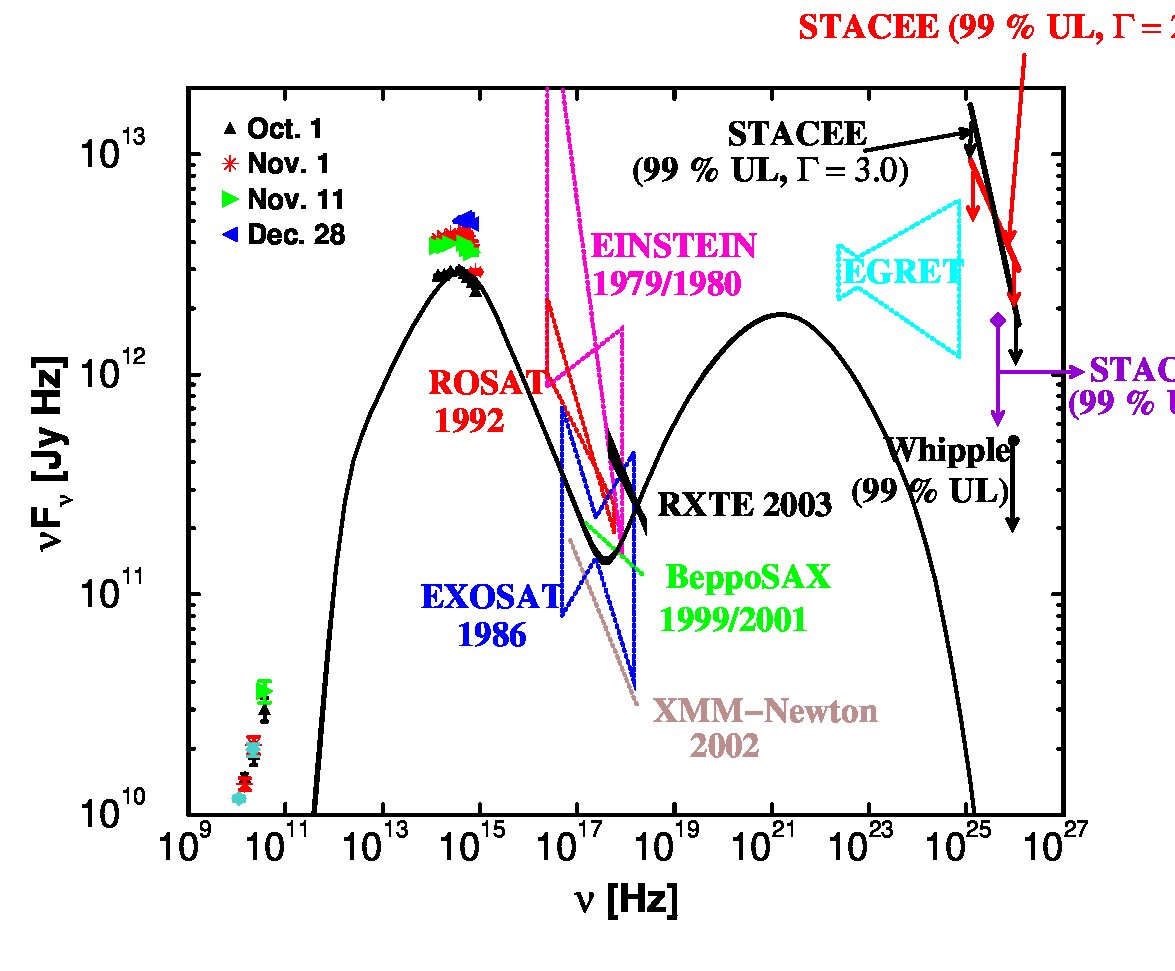 Figure 1
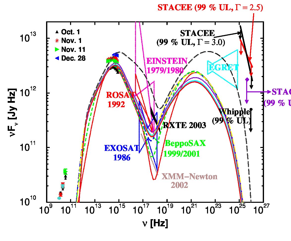 Figure 2
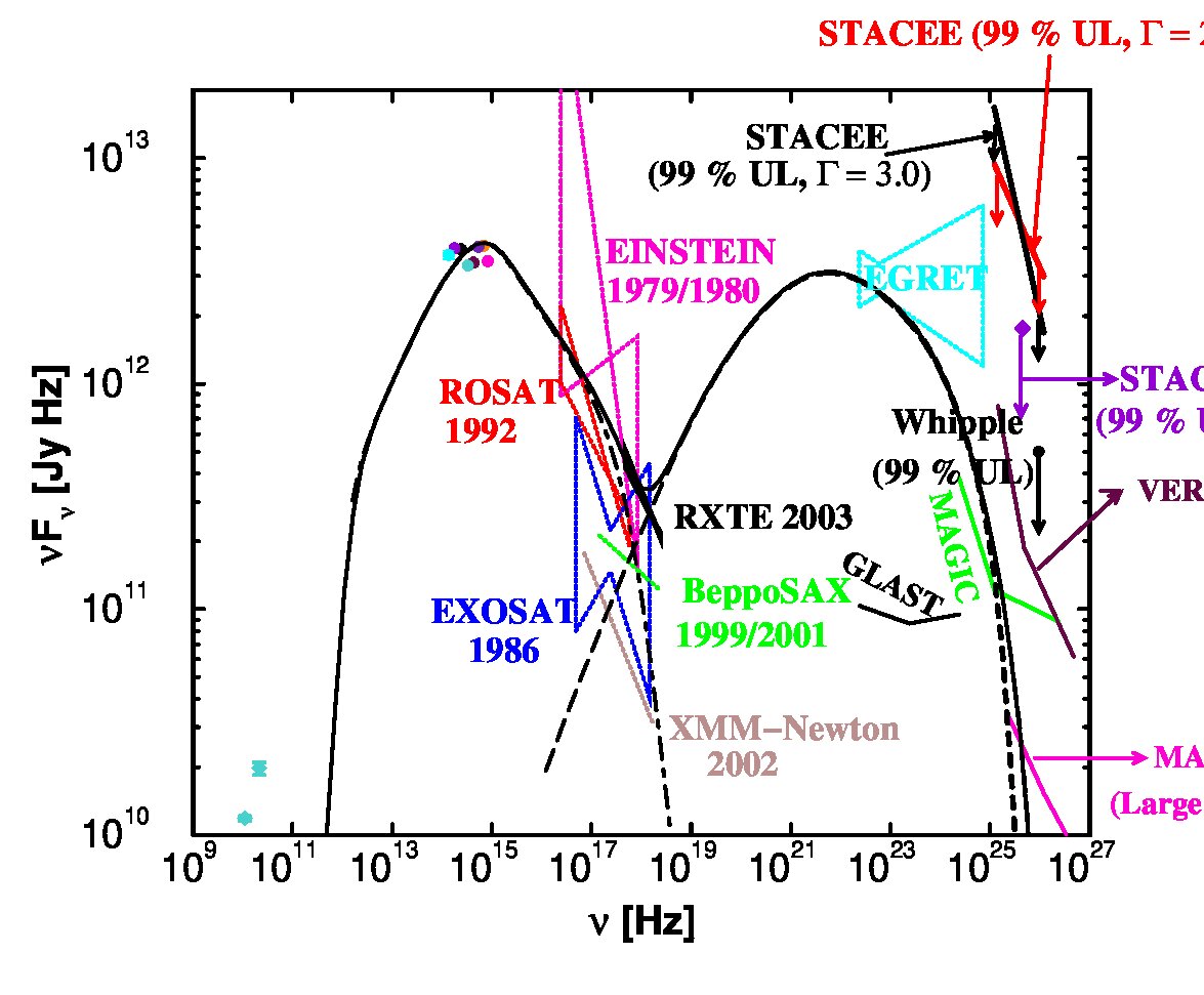 Figure 3
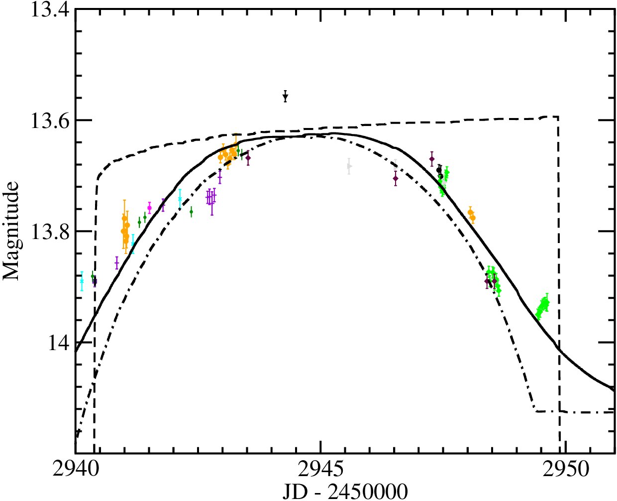 Figure 4
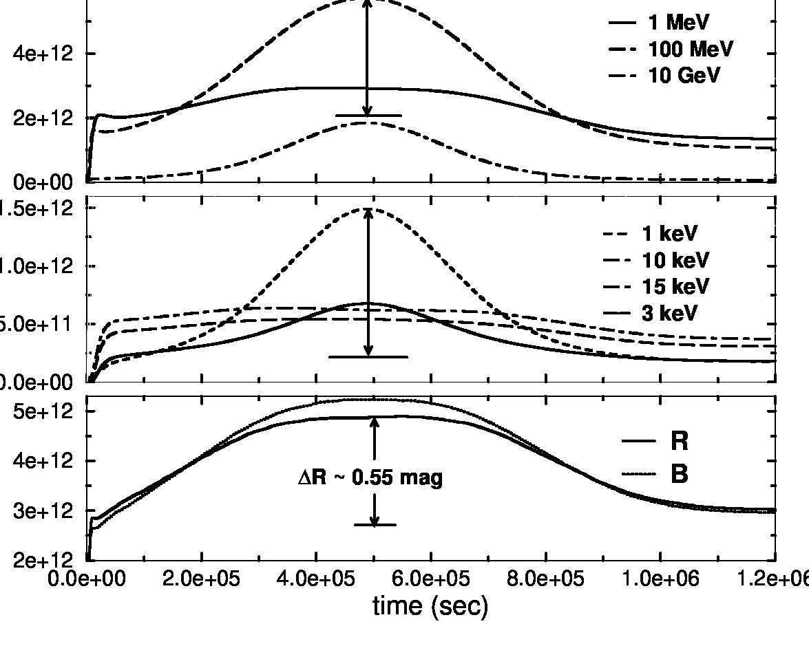 Figure 5
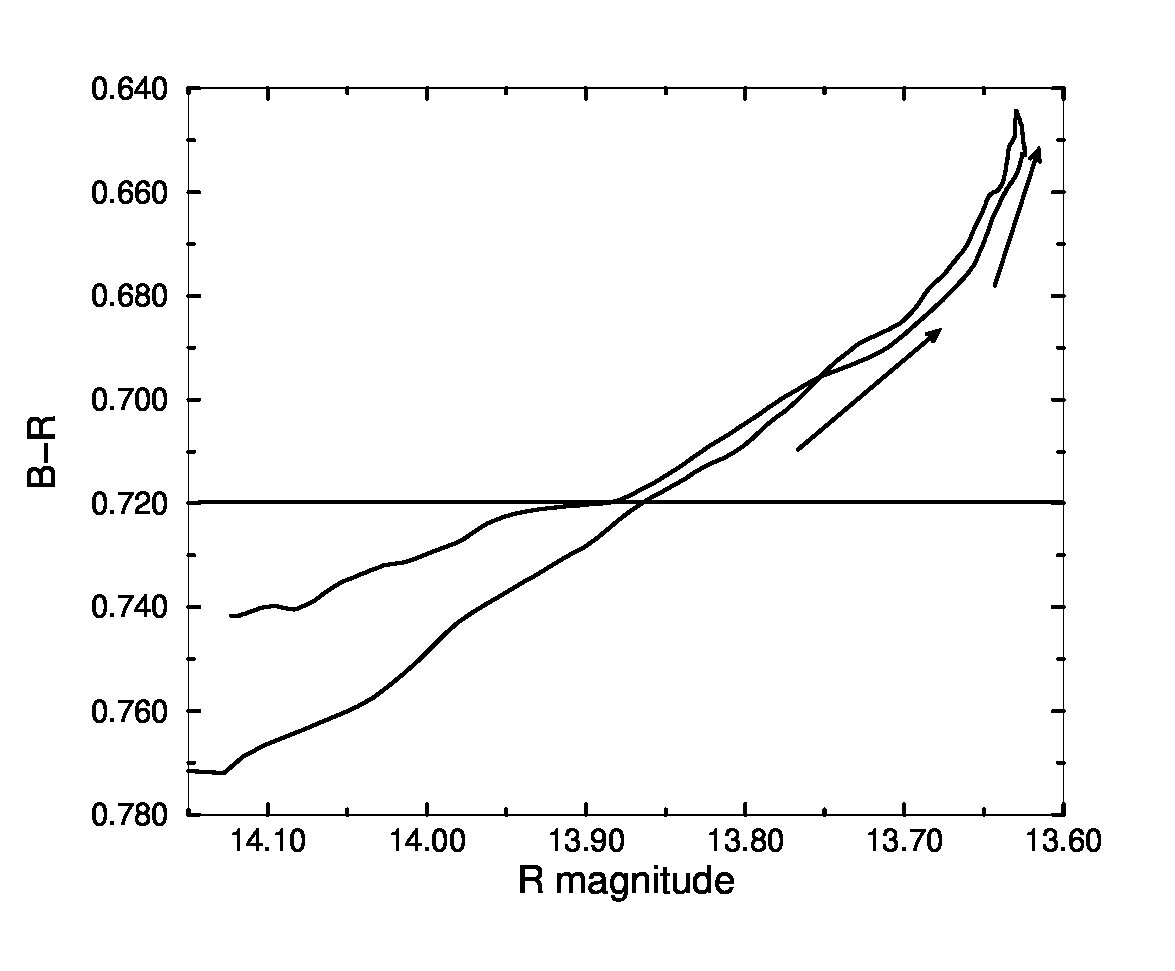 Figure 6
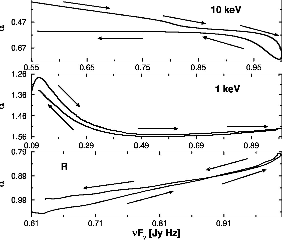 Figure 7
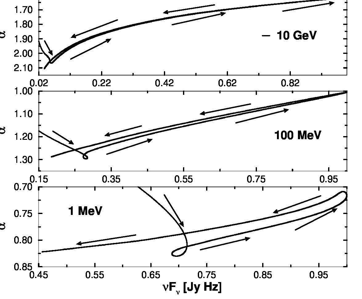 Figure 8
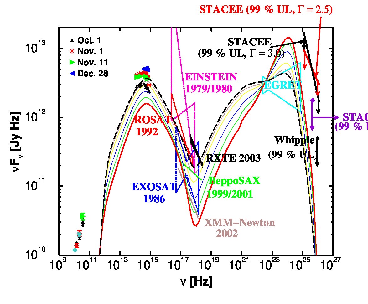 Figure 9
| Fit | [ ergs/s] | [] | [] | q | Profile | B [G] | [ cm] | [deg] | |||
|---|---|---|---|---|---|---|---|---|---|---|---|
| 1 | 2.7 | 1.8 | 3.0 | 3.1 | ——– | 1 | 2.4 | 24 | 3.59 | 2.4 | 0 |
| 2 | 8.0 | 2.1 | 4.5 | 2.4 | Gaussian | 1 | 2.8 | 24 | 3.59 | 2.4 | 0 |
| 3 | 8.0 | 2.1 | 4.5 | 2.4 | Gaussian | 1 | 2.8 | 24 | 3.59 | 2.4 | 0.3 |
Peer Reviews
No public reviews on file for this paper yet. If you reviewed it on a platform where reviews are public (OpenReview, ICLR, NeurIPS, ICML), you can paste yours below so the community can read it here.
Videos
No videos yet. Explain this paper in a talk, walkthrough, or lecture? Add one.
Modeling the Spectral Energy Distribution and Variability of 3C 66A
during the WEBT campaign of 2003 – 2004
M. Joshi11affiliation: Astrophysical Institute, Department of Physics and Astronomy,
Ohio University, Athens, OH 45701, USA and M. Böttcher11affiliation: Astrophysical Institute, Department of Physics and Astronomy,
Ohio University, Athens, OH 45701, USA
Abstract
The BL Lac object 3C 66A was observed in an extensive multiwavelength monitoring campaign from July 2003 till April 2004. The spectral energy distribution (SED) was measured over the entire electromagnetic spectrum, with flux measurements from radio to X-ray frequencies and upper limits in the very high energy (VHE) -ray regime. Here, we use a time-dependent leptonic jet model to reproduce the SED and optical spectral variability observed during our multiwavelength campaign. Our model simulations could successfully reproduce the observed SED and optical light curves and predict an intrinsic cutoff value for the VHE -ray emission at 4 GeV. The effect of the optical depth due to the intergalactic infrared background radiation (IIBR) on the peak of the high-energy component of 3C 66A was found to be negligible. Also, the presence of a broad line region (BLR) in the case of 3C 66A may play an important role in the emission of -ray photons when the emission region is very close to the central engine, but further out, the production mechanism of hard X-ray and -ray photons becomes rapidly dominated by synchrotron self-Compton emission. We further discuss the possibility of an observable X-ray spectral variability pattern. The simulated results do not predict observable hysteresis patterns in the optical or soft X-ray regimes for major flares on multi-day time scales.
galaxies: active — BL Lacertae objects: individual (3C 66A) — gamma-rays: theory — radiation mechanisms: non-thermal
††slugcomment: Submitted to The Astrophysical Journal
1 Introduction
Blazars are the most extreme class of Active Galactic Nuclei (AGN) exhibiting rapid variability at all wavelengths and a high degree of linear polarization in the optical. They have been observed at all wavelengths, from radio through VHE -rays and are characterized by non-thermal continuum spectra and radio jets with individual components often exhibiting apparent superluminal motion. This class of AGNs is comprised of BL Lac objects and flat-spectrum radio quasars (FSRQs), which are distinguished primarily on the basis of the absence or presence of broad emission lines in their optical spectra.
The broadband spectra of blazars are associated with non-thermal emission and exhibit two broad spectral components. The low energy component is due to synchrotron emission from non-thermal electrons in a relativistic jet whereas the high energy component is attributed either to the Compton upscattering of low energy radiation by the synchrotron emitting electrons (for a recent review see, e.g., Böttcher (2006)) or the hadronic processes initiated by relativistic protons co-accelerated with the electrons (Mücke & Protheroe, 2001; Mücke et al., 2003) . Blazars are often known to exhibit variability at all wavelengths, varying on time scales from months, to a few days, to even less than an hour in some cases. The radio emission of blazars shows variability on a time scale of weeks to months whereas the optical emission for some blazars might vary on a time scale of around one and a half hours. At X-ray energies, some HBLs exhibit characteristic loop features when the photon energy spectral index, , is plotted against the X-ray flux. These plots are known as hardness-intensity diagrams (HIDs) and the loop structures are called spectral hysteresis. This spectral hysteresis can be interpreted as the signature of synchrotron radiation, due to the gradual injection and/or acceleration of ultrarelativistic electrons in the emitting region and their subsequent radiative cooling (Kirk et al., 1998; Georganopoulos & Marscher, 1998; Kataoka et al., 2000; Kusunose et al., 2000; Li & Kusunose, 2000; Böttcher & Chiang, 2002).
3C 66A is classified as a low-frequency peaked (or radio selected) BL Lac object (LBL). The peak of the low-frequency component of LBLs generally lie in the IR or optical regime, whereas the high-energy component peak is located at several GeV, and the -ray output is typically comparable to or slightly higher than the spectral output of the synchrotron component. The redshift of 3C 66A has a relatively uncertain determination of (Bramel et al., 2005). It has exhibited rapid microvariability at optical and near infrared in the past and has been suggested as a promising candidate for detection by the new generation of atmospheric Čerenkov telescope facilities like H.E.S.S., MAGIC, or VERITAS (Costamante & Ghisellini, 2002). This object has been studied in radio, IR, optical, X-rays and -rays in the past. Its low-frequency component is known to peak in the IR - UV regime whereas the high-frequency component generally peaks at multi MeV - GeV energies. The multiwavelength SED and correlated broadband spectral variability behaviour of 3C 66A have been very poorly understood. For this reason, Böttcher et al. (2005) organized an intensive multiwavelength campaign to observe this object from July 2003 through April 2004, with the core campaign period being Sept. - Dec. 2003.
As described in Böttcher et al. (2005), the object exhibited several outbursts in the optical. The variation was on the order of m 0.3-0.5 over a timescale of several days. The minimum variability timsecale of 2 hr provided an estimate for the size of the emitting region to be on the order of cm. The optical flares suggested the presence of an optical spectral hysteresis pattern with the B - R hardness peaking several days before the R- and B- band flux peaked. The RXTE PCA data indicated a transition between the synchrotron and the high-energy component at photon energies of keV. The broadband SED of 3C 66A suggested that the synchrotron component peaked in the optical. In the VHE -ray regime, STACEE provided an upper limit at GeV whereas an upper limit at GeV resulted from simultaneous Whipple observations.
In this paper, we use a leptonic jet model to reproduce the broadband SED and the observed optical spectral variability patterns of 3C 66A and make predictions regarding observable X-ray spectral variability patterns and -ray emission. In §2, we describe the time-dependent leptonic jet model used to reproduce the observed SED and optical spectral variability patterns of 3C 66A. The parameters used to simulate the observed results are described in §3. The modeling results and VHE -ray predictions are discussed in §4. We summarize in §5.
Throughout this paper, we refer to as the energy spectral index, [Jy] . A cosmology with , , and km s*-1* Mpc*-1* is used. In this cosmology, and using the redshift of , the luminosity distance of 3C 66A is Gpc.
2 Model Description
The SEDs and optical variability patterns of 3C 66A were modeled using a one-zone homogeneous leptonic jet model. The model assumes injection of a population of ultrarelativistic non-thermal electrons and positrons into a spherical emitting volume (the “blob”) of comoving radius at a time-dependent rate. Since the positrons lose equal amount of energy as the electrons via the same radiative loss mechanisms so we do not distinguish between them throughout the paper. The injected electron population is described by a single power law distribution with a particle spectral index q, comoving injection density () and low- and high-energy cutoffs and , respectively, such that for , where is the injection function and is given by,
[TABLE]
where specifies the power of the injected pair population and is the blob volume in the comoving frame.
The randomly oriented magnetic field B has uniform strength throughout the blob and is determined by an equipartition parameter / (in the comoving frame), where is the magnetic field energy density and is the electron energy density. We keep constant so that the magnetic field value changes according to the evolving electron energy density value as determined by equation 5. The initial injection of the electron population into the blob takes place at a height above the plane of the central accretion disk. The emitting region travels relativistically with a speed along the jet. The jet is directed at an angle with respect to the line of sight. The Doppler boosting of the emission region with respect to the observer’s frame is determined by the Doppler factor , where is the bulk Lorentz factor.
As the emission region propagates in the jet, the electron population inside the blob continuously loses its energy due to synchrotron emission, Compton upscattering of synchrotron photons (SSC) and/or Compton upscattering of external photons (EC). The seed photons for the EC process include the UV soft X-ray emission from the disk entering the jet either directly (Dermer et al., 1992; Dermer & Schlickeiser, 1993) or after getting reprocessed in the BLR or other circumnuclear material (Sikora et al.,, 1994; Dermer et al., 1997). The time-dependent evolution of the electron and photon population inside the emission region is governed, respectively, by,
[TABLE]
and
[TABLE]
Here, is the radiative energy loss rate, due to synchrotron, SSC and/or EC emission, for the electrons. is the sum of external injection and intrinsic pair production rate and is the electron escape time scale. and are the photon emission and absorption rates corresponding to the electrons’ radiative losses and, is the photon escape timescale. The time-dependent evolution of the electron and photon population inside the blob is followed and radiative energy loss rates as well as photon emissivities are calculated using the time-dependent radiation transfer code of Böttcher & Chiang (2002).
The model only follows the evolution of the emission region out to sub-pc scales and as a result only the early phase of -ray production can be simulated. Since the radiative cooling is strongly dominant over adiabatic cooling during this phase and the emission region is highly optically thick out to GHz radio frequencies, the simulated radio flux is well below the actual radio data. We do not simulate the phase of the jet components in which they are expected to gradually become transparent to radio frequencies as that would require the introduction of several additional, poorly constrained parameters.
3 Model Parameters
The model independent parameters that were estimated using the SED and optical intraday variability measurements (see Böttcher et al., 2005) were used to develop an initial set of input parameters:
[TABLE]
Here p is the equilibrium spectral index that determines the optical synchrotron spectrum and for strongly cooled electrons. The initial set of parameters was modified to reproduce the quiescent as well as the flaring state of 3C 66A. Approximately 350 simulations were carried out to study the effects of variations of various parameters, such as , , q, B and , on the resulting broadband spectra and light curves. The set of model parameters that provided a satisfactory fit to the quiescent state of 3C 66A involved a value of the Doppler factor, and a viewing angle of . These parameters were chosen on the basis of VLBA observations that provided the limits on the superluminal motion and indicated bending of the jet towards the line of sight thus resulting in a smaller viewing angle and a higher Doppler boosting of the emission region as compared to the values inferred from the superluminal measurements on larger scales (Jorstad et al., 2005; Böttcher et al., 2005). The fitting of the SED both in the quiescent as well as flaring state of 3C 66A was carried out such that the simulated quiescent state does not overpredict the X-ray photon flux as X-ray photons are expected to be dominated by the flaring episodes. On the other hand, the flaring state was simulated such that the resulting time-averaged spectrum passes through the observed time-averaged optical as well as X-ray data points. This was achieved by varying individual parameters, such as, , and q between the values for quiescent and flaring states with time profiles as discussed in the next section. A value of , and provided a satisfactory fit to the flaring state. Also, during our multiwavelength campaign of 2003 - 2004, flux upper limits at multi-GeV - TeV energies could be obtained and as a result we could get upper limits on the respective parameters governing the EC component. The various model parameters used to simulate the two states of 3C 66A are listed in Table 1.
Figures 1 and 2 respectively show the reproduction of the SED of 3C 66A, for both the quiescent and flaring state observed during the campaign period. The quiescent state is a reproduction of the state observed around 1st October 2003 whereas the flaring state is the reproduction of a generic 10 day flaring period corresponding to the timescale of several of the major outbursts that were observed during the campaign. The simulated time-averaged spectrum of 3C 66A in the flaring state is shown in Figure 3. The simulations, corresponding to fits 1 and 2 of Table 1, were carried out for a pure SSC emission process by artificially setting , where is the bolometric disk luminosity. Fit 3 of Table 1 refers to an EC+SSC case with and is shown in Figure 9. The value of was chosen such that it is more than the value of the jet luminosity used in the simulations and at the same time does not produce a blue bump in the simulated SED. In order to assess the possible effect of EC emission in 3C66A, an upper limit to the optical depth of the BLR was first determined using XSTAR, which returns the ionization balance and temperature, opacity, and emitted line (, ) and continuum fluxes. The BLR was modeled as a spherical shell with pc and pc, where and stand for the inner and outer radii of the broad line region. A Thomson optical depth of 0.3 for the BLR was chosen as a reasonable upper limit such that the line emission is weak enough or absent to be consistent with the observed featureless continuum.
4 Results and Discussion
As can be seen in Figure 3, the time-averaged simulated spectrum passes through the time-averaged optical data points whereas the high energy end of the synchrotron component passes through the time averaged X-ray data indicating the dominance of synchrotron emission in the production of such photons in case of flaring. For X-ray photons with energy beyond 10-12 keV, the data is less reliable due to low count rates and possible source confusion with 3C 66B. The spectral upturn at 7 keV occurs due to the presence of the SSC component in the simulation. The presence of this component cannot be suppressed because in order to suppress it the population of seed photons would have to be diluted, which can be done by increasing the size of the emission region. But the size of the emission region cannot be increased any further due to the strict constraint on the maximum size of the blob that comes from the observed minimum variability timescale in the optical region, which is 2 hrs. Hence, the emission region size cannot exceed cm. Thus, our model suggests that the harder X-ray photons come from the SSC and not the synchrotron mechanism with the expected spectral hardening taking place at 7 keV. The high energy component, due to the SSC emission, for the time-averaged spectrum (see Figure 3) cuts off at Hz or 4 GeV. From the simulated level of VHE emission we predict that the object is well within the observational range of MAGIC, VERITAS and, especially, GLAST (see Figure 3) whose sensitivity limit is 50 times lower than that of EGRET at 100 MeV and even more at higher energies and its two year limit for source detection in an all-sky survey is (at energies MeV). Thus it will be possible to extract the spectral and variability information for this object at such high energies in future observations.
Flaring above the quiescent state of 3C 66A was reproduced using a flaring profile for the electron injection power () that was Gaussian in time (see Figure 4):
[TABLE]
Here, qu and fl stand for the quiescent and flaring state respectively, z determines the position of the emission region in the jet at time t, indicates the position of the center of the simulated flare and stands for the Gaussian width of the flare.
The rest of the parameters such as and and q were also changed accordingly. In order to simulate the observed optical flare, the system was first allowed to come to an equilibrium and after the equilibrium was set up the flare was introduced with a Gaussian width, corresponding to 14 days in the observer’s frame. Although the flare was introduced in order to simulate the observed major optical outbursts lasting for 10 days, the choice of 14 days for the Gaussian width was made such that the width of the simulated flare matches that of the observed flare, was adjusted such that the centre of the simulated flare aligns with that of the observed one and the value of was varied such that the peak of the simulated flare matches that of the observed one.
The observed lightcurves did not agree well with a flaring profile that was top-hat or triangular in time as can be seen in the figure. The presence of a flare that is Gaussian in time might represent an initial injection of particles into the emission region at the base of the jet. The particles slowly get accelerated as a shock wave ploughs through the region and finally dies out in time. Crucial information on the dominant acceleration mechanism comes from the change in the shape of the particle injection spectral index with time, which might also indicate a possible change in the B-field orientation. According to the current understanding of acceleration mechanisms, parallel shocks generally produce electron spectra of with (Achterberg et al., 2001; Galant et al., 1999), whereas oblique shocks produce much softer injection spectral indices. On the other hand, 2nd order Fermi acceleration behind the shock front might give rise to a harder injection index of the order of or beyond (Virtanen & Vainio, 2005). In order to reproduce the flaring state, the simulation first starts out in the quiescent state with quiescent state parameters and then the value of these parameters is changed to the flaring state parameters as the flaring is introduced in the simulation. Since, the value of q, in our simulations, changes from 3.1 (quiescent state) to 2.4 (flaring state) it might indicate a possible change in the orientation of the B-field from oblique to parallel during the flaring episode or an interplay between the 1st and 2nd order Fermi acceleration thereby making the particle spectra harder. The contribution from such acceleration mechanisms and the shear acceleration (Rieger & Duffy, 2004) might play an important role in accelerating the particles to higher energies.
The simulated optical variability in the R band (0.55 mag) matches the observed value (0.3-0.5 mag) for a 10 day period outburst. The predicted variability in B is more than that of R by mag as also observed, which indicates that the spectrum is becoming harder (see Figure 5) with the spectral upturn occuring at B-R 0.72 mag as shown in Figure 6. Figure 6 is a hardness intensity graph that shows that the object follows a positive correlation of becoming harder in B-R while getting brighter in both the bands during the 10-day flare simulated in Figure 2. This agrees well with the observed optical variability pattern. In this study, we are not addressing the variability that was observed on intraday timescales as that analysis would open up an even larger parameter space, which cannot be reasonably well constrained without any variability information in the X-ray regime.
The flare declines faster as compared to the time taken by the flare to rise. This might indicate that the particles’ synchrotron cooling timescale is less than or equal to the light crossing time.
[TABLE]
We can calculate the observed synchrotron cooling timescale, in the optical regime from equation 14 (Böttcher et al., 2005) using , and for the quiescent state and and for the flaring state (see Figures 1 and 2), where is the characteristic synchrotron frequency in units of Hz. This yields a value of hours for the quiescent state whereas for the flaring state it reduces to 37 minutes. The observed minimum variability timescale of 2 hours might therefore correspond to the observed dynamical timescale, where
[TABLE]
This implies that it takes time to build up the electron population in the emission region through flaring but once built up the electrons lose their energy efficiently to produce synchrotron photons. This can be used to constrain the value of the magnetic field in the jet, which has been allowed to evolve in time keeping and has an average value of 2.4 Gauss in the simulated quiescent state and 2.8 Gauss in the simulated flaring period.
The crossover of X-ray lightcurves, in our simulations, is a result of the dominance of the SSC component in hard X-rays (see Figure 5). The lightcurve of soft X-ray photons of energy 1 keV exhibits a greater variability of Jy Hz in its flux as compared to their optical counterpart. This is expected because the soft X-ray photons, during the flaring episode, are produced from synchrotron emission of electrons that are accelerated to very high energies and as a result have a very short cooling timescale and thus greater variability. In case of hard X-rays no significant variability is predicted. This is because such photons are produced from Compton upscattering of synchrotron photons off the low-energy electrons and as a result the cooling timescale is much longer as compared to the cooling timescale of their soft X-ray and optical counterparts. Hence, the variability information gets washed out. The predicted X-ray spectral variability pattern of large variability in the low X-ray energy band and negligible variability in the high X-ray energy band is similar to what has also been observed in BL Lacertae on several occasions (see for e.g., Ravasio et al., 2003, 2002).
As can be seen in Figure 7, spectral hysteresis patterns are not predicted for optical as well as soft X-ray photons. This is expected because the cooling timescale of their parent electron population is so short that what is observed is the average effect of this cooling over the dynamical timescale and hence any hysteresis pattern gets smeared out. On the other hand, one expects to see these patterns at higher energies because as explained earlier, this photon population comes from Compton upscattering off low-energy electrons, which have a longer cooling timescale and as a result the photon population gradually builds up over time and then dies away giving rise to a hysteresis pattern (see Figure 8). The slight spectral softening at 10 keV seen in its hysteresis pattern (see Figure 7) for higher values of indicates a small synchrotron contribution near the peak of the flare.
The simulated instantaneous SED, for a pure SSC model, shows a definite presence of -ray emission in 3C66A, in the quiescent as well as the flaring state (see Figure 1 and 2). The intrinsic cutoff of VHE emission in the flaring state, according to the simulations, for the time averaged spectrum is Hz or 4 GeV. In our simulations, the emission of VHE -ray photons is produced by the SSC mechanism in the quiescent as well as the flaring state. Figure 5 shows the simulated lightcurves for VHE photons and as can be seen the value changes by Jy Hz at 100 MeV. The variability in VHE photons is expected as they are the result of Compton upscattering off the higher energy electrons and due to this the hysteresis pattern is not seen at such high energies as the cooling timescale of such high energy electrons is very short (see Figure 8).
From Figure 9, it can be seen that the high-energy component of 3C 66A, in the flaring state, could start out with a dominant contribution of the EC emission, shown by the red solid line. But as the blob travels further away and passes the outer edge of the broad line region, the EC contribution becomes less significant and the SSC emission takes over. This is indicated by the black long-dashed line in the figure. We might actually find that this maximum contribution would be just enough to explain the historical EGRET flux and that there could be GeV flaring due to early external Comptonization.
The effect of an optical depth due to the IIRB on the spectra of 3C 66A was also evaluated and was found to be insignificant in the energy range we are interested in as shown in Figure 3. The optical depth due to the IIRB was determined using the analytic expression given in Stecker et al. (2006). The absorption till GeV is negligible and becomes slightly observable at 200 GeV as the optical depth takes a value of, 2.9. Hence, the SSC emission cutoff value at 4 GeV is intrinsic.
5 Summary
An extensive analysis of the data of 3C 66A, obtained from the multiwavelength monitoring campaign on 3C 66A from July 2003 to April 2004, was carried out using a time-dependent leptonic jet model. The analysis was targeted towards understanding the dominant radiation mechanism in the production of the high-energy component of the SED of 3C 66A in the quiescent as well as the flaring state. Our simulations yielded predictions regarding the observable variability patterns in the X-ray as well as the VHE energy regimes where such patterns could not be detected during the campaign. The object was well sampled in the optical, especially in the R-band, during the campaign. It had exhibited several major outbursts (10 days) in this regime with a varibility of m 0.3-0.5. The X-ray data covered the 3-10 keV range with the onset of the high-energy component expected at 10 keV photon energies. Only upper limits in the VHE regime had been obtained.
The simulations from our model could successfully reproduce the observed SED as well as the optical spectral variability patterns. The model suggests the dominance of the SSC mechanism in the production of hard X-ray as well as VHE photons. On the other hand, soft X-ray photons exhibit spectral softening during flaring indicating the onset of the synchrotron component in this energy range. According to the simulated time-averaged spectrum, the synchrotron component is expected to cut off near 7 keV whereas the SSC component cuts off at 4 GeV.
A flaring profile that was Gaussian in time could successfully reproduce the observed flaring profile for a timescale of 10 days. The simulated varibility in R (m 0.55) agreed well with the observed variability. According to the simulations, the object flares up in R and B simultaneoulsy with (37 minutes) being less than or equal to the light crossing time (2 hours) during flaring. No significant variability is predicted in the hard X-ray regime. This is due to the production of such photons from Compton upscattering off low-energy electrons with cooling timescales much longer than the light crossing time, . On the other hand, the simulated lightcurves of VHE -ray photons exhibit significant variability as such photons are produced from the Compton upscattering off higher energy electrons with shorter cooling timescales than the light crossing time.
The effect of the optical depth due to absorption by the IIBR on the SED of 3C 66A was also evaluated. The simulations do not predict a significant effect on the SED due to the optical depth. The SSC emission cutoff predicted to be at 4 GeV can be taken as the intrinsic SSC emission cutoff value for this object. We predict the object to be well within the observational range of MAGIC, VERITAS and GLAST. Finally, the EC emission for this object was also calculated and it appears that the EC emission could be dominant in the high-energy component initially, but as the emission region travels further away from the BLR, the EC contribution becomes less significant and the SSC emission takes over. It is highly probable that this maximum contribution of the EC component might explain the historical EGRET flux and that there could be GeV flaring due to early external Comptonization.
This work was partially supported through NRL BAA 76-03-01, contract no. N00173-05-P-2004.
The reference list from the paper itself. Each links out to its DOI / PubMed record.
- 1Achterberg et al. (2001) Achterberg, A., et al., 2001, MNRAS, 328, 393
- 2Böttcher (2006) Böttcher, M., 2006, in proc. “The Multi-Messenger Approach to High-Energy Gamma-Ray Sources”, Barcelona, Spain, 2006, Astroph. & Space Sci., in press
- 3Böttcher et al. (2005) Böttcher, M., et al., 2005, Ap J, 631, 169
- 4Böttcher & Chiang (2002) Böttcher, M., & Chiang, J., 2002, Ap J, 581, 127
- 5Böttcher et al. (1997) Böttcher, M., Mause, H., & Schlickeiser, R., 1997, A&A, 324, 395
- 6Bramel et al. (2005) Bramel, D. A., et al., 2005, Ap J, 629, 108
- 7Costamante & Ghisellini (2002) Costamante, L., & Ghisellini, G., 2002, A&A, 384, 56
- 8Dermer et al. (1997) Dermer, C. D., Sturner, S. J., & Schlickeiser, R., 1997, Ap JS, 109, 103