Orbifold cohomology of abelian symplectic reductions and the case of weighted projective spaces
Tara S. Holm

TL;DR
This paper explores the topology and orbifold cohomology of symplectic quotients, especially weighted projective spaces, demonstrating simplified computational methods and providing new explicit cohomology ring calculations.
Contribution
It introduces direct computational techniques for orbifold cohomology of abelian symplectic reductions, specifically for weighted projective spaces, bypassing complex combinatorial tools.
Findings
Computed Chen-Ruan orbifold cohomology rings for weighted projective spaces
Demonstrated simplified methods for topological computations in symplectic quotients
Compared different cohomology rings associated with weighted projective spaces
Abstract
These notes accompany a lecture about the topology of symplectic (and other) quotients. The aim is two-fold: first to advertise the ease of computation in the symplectic category; and second to give an account of some new computations for weighted projective spaces. We start with a brief exposition of how orbifolds arise in the symplectic category, and discuss the techniques used to understand their topology. We then show how these results can be used to compute the Chen-Ruan orbifold cohomology ring of abelian symplectic reductions. We conclude by comparing the several rings associated to a weighted projective space. We make these computations directly, avoiding any mention of a stacky fan or of a labeled moment polytope.
Click any figure to enlarge with its caption.
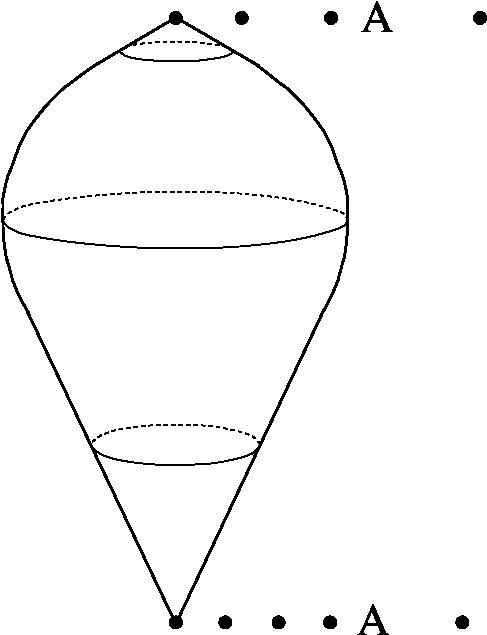 Figure 1
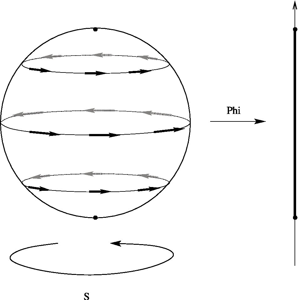 Figure 2
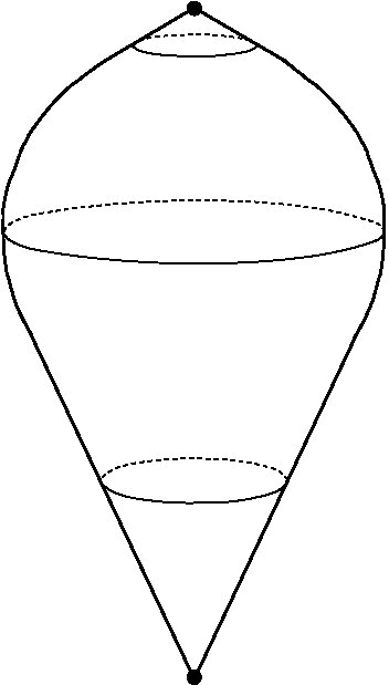 Figure 3
Peer Reviews
No public reviews on file for this paper yet. If you reviewed it on a platform where reviews are public (OpenReview, ICLR, NeurIPS, ICML), you can paste yours below so the community can read it here.
Videos
No videos yet. Explain this paper in a talk, walkthrough, or lecture? Add one.
Taxonomy
TopicsHomotopy and Cohomology in Algebraic Topology · Advanced Algebra and Geometry · Algebraic Geometry and Number Theory
Orbifold cohomology of abelian symplectic reductions and the case of weighted projective spaces
Tara S. Holm
Department of Mathematics, Cornell University, Ithaca, NY 14853-4201 USA
Abstract.
These notes accompany a lecture about the topology of symplectic (and other) quotients. The aim is two-fold: first to advertise the ease of computation in the symplectic category; and second to give an account of some new computations for weighted projective spaces. We start with a brief exposition of how orbifolds arise in the symplectic category, and discuss the techniques used to understand their topology. We then show how these results can be used to compute the Chen-Ruan orbifold cohomology ring of abelian symplectic reductions. We conclude by comparing the several rings associated to a weighted projective space. We make these computations directly, avoiding any mention of a stacky fan or of a labeled moment polytope.
Key words and phrases:
Symplectic quotient, orbifold, cohomology
1991 Mathematics Subject Classification:
Primary 53D20; Secondary 14N35, 53D45, 57R91
TSH is grateful for the support of the NSF through the grant DMS-0604807.
Contents
- 1 Symplectic manifolds and quotients
- 2 Orbifolds and their cohomology
- 3 Why the symplectic category is convenient
- 4 The case of weighted projective spaces
The notion of an orbifold has been present in topology since the 1950’s [S1, S2]. More recently, orbifolds have played an important role in differential and algebraic geometry, and in mathematical physics. A fundamental theme is to compute topological invariants associated to an orbifold, with one ostensible goal to understand Gromov-Witten invariants for these spaces. The aim of the present article is modest: to expound how techniques from symplectic geometry may be used to understand the degree-zero genus-zero Gromov-Witten invariants with three marked points, the so-called Chen-Ruan orbifold cohomology ring; and to make explicit the details of these techniques in the case of weighted projective spaces.
In the symplectic category, orbifolds arise as symplectic quotients. We recount the techniques from symplectic geometry that may be used to compute topological invariants of a symplectic quotient. This is based on Kirwan’s seminal work [Ki]; and for orbifold invariants, the author’s joint work with Goldin and Knutson [GHK]. The quotients we consider are by a compact connected abelian group. We employ techniques coming from algebraic topology, most notably using equivariant cohomology. For those used to working with finite groups, it is important to note that, whereas for finite groups the invariant part of a cohomology ring is identical to the equivariant cohomology, this is not the case for connected groups.
The main example in this article is a weighted projective space . Its definition depends on a sequence of positive integers. Kawasaki showed that the ordinary cohomology groups, with integer coefficients, of the underlying topological space of a weighted projective space are identical to the cohomology groups of a smooth projective space [Ka], but there is a twisted ring structure. We review the details of his work. Then in Theorem 4.2, we compute the cohomology of the orbifold , proving that
[TABLE]
Whereas Kawasaki finds a twist in the the ring structure, we find torsion in high degrees of the ring (0.1). There is a natural map from Kawasaki’s ring to this one, and we describe the map explicitly. Finally in Theorem 4.3, we compute the Chen-Ruan cohomology ring of this orbifold. We make this computation using integer coefficients, generalizing results in [J, Ma1, Ma2]. Moreover, we give explicit generators and relations, and avoid mentioning a stacky fan [BCS] or a labeled polytope [LT, GHK].
The definitions in this article make sense for arbitrary coefficient rings. Indeed, all computations in the final section use integer coefficients. Moore and Witten have suggested that the torsion in -theory has more physical significance than torsion in cohomology [MoWi]. The author together with Goldin, Harada and Kimura, is investigating a -theoretic version of [GHK] and of the computations herein, building on the work of Harada and Landweber [HL].
The remainder of the paper is organized as follows. In Section 1 we give a quick exposition of how orbifolds arise in the symplectic category. We then introduce several cohomology rings associated to an orbifold in Section 2. We advertise the ease of computation for these rings in Section 3. The novel results in this article are the computations in Section 4. We include detailed proofs that avoid much of the symplectic machinery used in [GHK].
Acknowledgments. Many thanks are due to Tony Bahri, Matthias Franz, Rebecca Goldin, Megumi Harada, Ralph Kaufmann, Takashi Kimura, Allen Knutson, Eugene Lerman, Reyer Sjamaar, and Alan Weinstein for many helpful conversations; and to Yoshiaki Maeda and the organizers and sponsors of Poisson 2006 in Tokyo, Japan, where this work was presented.
1. Symplectic manifolds and quotients
We begin with a very brief introduction to the symplectic category; a more detailed account of the subject can be found in [CdS]. A symplectic form on a manifold is a closed non-degenerate two-form . Thus, for any tangent vectors , . The key examples include the following.
Example 1.1:
with equal to the signed area of the parallelogram spanned by and . This is the Fubini-Study form on .
Example 1.2:
any orientable Riemann surface with as in Example 1.1. Note that orientability is a necessary condition on a symplectic manifold , because the top exterior power of the symplectic form is a volume form.
Example 1.3:
with .
Example 1.4:
a coadjoint orbit of a compact connected semisimple Lie group, equipped with the Kostant-Kirillov-Soriau form.
Example 1.3 gains particular importance because of
Darboux’s Theorem 1.5.
Let be a symplectic -manifold with symplectic form . Then for every point , there exists a coordinate chart about with coordinates so that on this chart,
[TABLE]
Thus, whereas Riemannian geometry uses local invariants such as curvature to distinguish metrics, symplectic forms are locally indistinguishable.
The symmetries of a symplectic manifold may be encoded as a group action. Here we restrict ourselves to a compact connected abelian group . An action of on is symplectic if it preserves ; that is, , for each , where is the diffeomorphism corresponding to the group element . The action is Hamiltonian if in addition, for every , the vector field
[TABLE]
is a Hamiltonian vector field. That is, we require that is an exact one-form. Each is a smooth function on , determined up to a constant. Taking them together, we may define a moment map
[TABLE]
Returning to our examples, we have Hamiltonian actions in all but the second example.
Example 1.6:
The circle acts on by rotations. If we use angle and height coordinates on , then the vector field this action generates is tangent to the latitude lines, so in coordinates, , and since , , so a moment map is the height function on , as shown in Figure 1.1 below.
Example 1.7:
If is a two-torus , then acts on itself by multiplication. This action is symplectic, but is not Hamiltonian. In fact, no Riemann surface with non-zero genus has a nontrivial Hamiltonian torus action.
Example 1.8:
The torus acts by coordinate-wise multiplication on . This action rotates each copy of (at unit speed), and is Hamiltonian. Identifying , a moment map is
[TABLE]
up to a constant multiple.
Example 1.9:
Each coadjoint orbit may be identified as a homogenous space , where is a Levi subgroup of the Lie group . Thus and its maximal torus act on by left multiplication. A -moment map is inclusion
[TABLE]
and a -moment map is the -moment map composed with the natural projection that is dual to the inclusion .
In each of these examples, the image of the (torus) moment map is a convex subset of . This is true more generally.
Convexity Theorem 1.10 ([A],[GuSt]).
If is a compact Hamiltonian -space, then is a convex polytope. It is the convex hull of , the images of the -fixed points.
The convexity theorem is an example of a localization phenomenon: a global feature (the image of the moment map) that is determined by local features of the fixed points (their images under the moment map). The convexity property is a recurring theme in symplectic geometry; its many guises are illustrated in [GuSj].
The moment map is a -invariant map: it maps entire -orbits to the same point in . Thus when is a regular value, the level set is a -invariant submanifold of . Moreover, the action of on a regular level set is locally free: it has only finite stabilizers. This follows directly from the moment map condition: at a regular value, is never zero, implying that is not zero, so there is no -parameter subgroup fixing points in the level set. Thus, at a regular value the symplectic reduction is an orbifold. In fact, Marsden and Weinstein proved
Theorem 1.11 ([MaWe]).
If is a Hamiltonian -space and is a regular value of the moment map , then the symplectic reduction is a symplectic orbifold.
More generally, the symplectic reduction at a critical value is a symplectic stratified space [SL].
Symplectic reduction is an important technique for constructing new symplectic manifolds from old. From our examples, we may construct several classes of symplectic manifolds.
Example 1.12:
For the action of on by rotation, the level set of a regular value is a latitude line, which the circle rotates. The quotient is a point. Note that if acts by rotation at twice the usual speed, then the quotient, as an orbifold, is . Thus, every orbifold is a quotient of by a rotation action.
Example 1.13:
acts on by rotation of each copy of . The level set of a regular value is a copy of , and so again the quotient is a point (or potentially an orbipoint, for different actions of ). However, we may also restrict our attention to subtori . The action of is still Hamiltonian, and for certain choices of , is a symplectic toric orbifold. Lerman and Tolman show that every effective symplectic toric orbifold may be constructed in this way [LT].
Example 1.14:
For the -action on a coadjoint orbit , the symplectic reduction is known as a weight variety. One may determine the possible orbifold singularities by analyzing the combinatorics of and its Weyl group. See, for instance, [Kn] or [GHK]. This reduced space plays an important role in representation theory.
2. Orbifolds and their cohomology
We now turn to orbifolds in the topological category. In terms of local models, an orbifold is a topological space where each point has a neighborhood homeomorphic (or diffeomorphic) to the quotient of a (fixed dimensional) vector space by a finite group. Satake introduced this notion in the 1950’s [S1, S2], originally calling the spaces -manifolds. Thurston coined the term orbifold when he rediscovered them in the 1970’s (see [Th]) in his study of -manifolds. This local model, however, makes it difficult to define very basic pieces in the theory of orbifolds: overlap conditions on orbifold charts, suborbifolds, and maps between orbifolds. As is evident already in the work of Haefliger [Hæ], the proper way to think of an orbifold is as a Morita equivalence class of groupoids, one of which is a proper étale groupoid (see [Moe]); or equivalently as a smooth Deligne-Mumford stack (see [DM]). For example, using this structure, a map of orbifolds should simply be a morphism of the appropriate objects.
While groupoids or stacks provide the correct mathematical framework, the technology is a bit beyond the scope of this article. Indeed, for us it is sufficient to work with the local models, largely because we restrict our attention to orbifolds that arise as global quotients. Nevertheless, we will need to distinguish between an orbifold or and its underlying topological space (or coarse moduli space) . In particular, when is presented as a global quotient of a manifold by a group , we will use square brackets to denote the orbifold, and to denote the underlying coarse moduli.
For an orbifold , at each point , we have a local isotropy group at . We will be interested in almost complex orbifolds, that is orbifolds that have local models isomorphic to , with a finite group acting unitarily on . Our main example in this section is the orbisphere shown in the figure below.
This is a symplectic toric orbifold in the sense of Tolman and Weitsman [LT]. In that context, it corresponds to the labeled polytope that is an edge, with the vertices labeled and . This orbifold cannot (always) be presented as a global quotient by a finite group, although it can be presented as a symplectic reduction. When and are relatively prime, it is the reduction of by the Hamiltonian -action
[TABLE]
Thus, it is a global quotient of the level set by a locally free action. In this case, it is also the global quotient of by a action111With an apology to number theorists, we take the topologist’s notation: denotes the integers modulo .. When and are not relatively prime, the orbisphere is not a global quotient by a finite group, but it is still a symplectic quotient of by a Hamiltonian action, where (following [LT]). Note also that an orbisphere is isomorphic to a weighted projective space exactly when and are relatively prime. If and are not relatively prime, the weighted projective space is not reduced: it has a global stabilizer. On the other hand, the orbisphere described above is always reduced.
Next we turn to algebraic invariants that we may attach to an orbifold . The hope is that these invariants are computable and at the same time retain some information of the orbifold structure of . All the invariants are isomorphic to singular cohomology if is in fact a manifold.
Definition 2.1.
The ordinary cohomology ring of an orbifold is the singular cohomology of the underlying topological space ,
[TABLE]
with coefficients in a commutative ring .
This ring is computable using standard techniques from algebraic topology, but it does not distinguish between the orbisphere in Figure 2.1 and a smooth sphere.
For the second invariant, we restrict our attention to orbifolds presented as the quotient of a manifold by the locally free action of a Lie group . It is conjectured that every orbifold can be expressed as such a global quotient, and it is known to be true for effective or reduced orbifolds, those that do not have a global finite stabilizer (see, for example, [EHKV, Theorem 2.18]). A presentation as a global quotient is desirable because then the topology or geometry of the quotient is simply the -equivariant topology or geometry of the manifold . This principle motivates the following definition.
Definition 2.2.
Given a presentation of an orbifold as a global quotient, the cohomology ring of the orbifold is the equivariant cohomology ring
[TABLE]
with coefficients in a commutative ring .
Recall that equivariant cohomology is a generalized cohomology theory in the equivariant category. Using the Borel model, we define
[TABLE]
where is a contractible (though infinite dimensional) space with a free action, and acts diagonally on . There are well-developed methods for computing equivariant cohomology, hence this invariant is still computable.
Whenever is a global quotient, the associated quotient map
[TABLE]
is a -invariant map. This induces a continuous map
[TABLE]
When is a manifold (i.e. acts on locally freely), this map is a fibration with fiber . The map induces a map in cohomology,
[TABLE]
This induced map is an isomorphism when
acts freely on ; 2. 2.
is a finite group and is a ring in which is invertible; and 3. 3.
acts locally freely on and is a field of characteristic [math].
This last item implies that the cohomology of the orbifold differs from the cohomology of its coarse moduli only in its torsion. Notably, when , this ring does in fact distinguish between the orbisphere in Figure 2.1 and a smooth sphere.
The third invariant was introduced by Chen and Ruan [CR] to explain mathematically the stringy Betti numbers and stringy Hodge numbers that physicists have attached to orbifolds. To define this third invariant, we need to introduce the first inertia orbifold
[TABLE]
This is again an orbifold, and is the suborbifold called the identity sector whose pairs consist of a point in together with the identity element coset. The other connected components of are called the twisted sectors. For a global quotient with abelian, we may identify . On the other hand, when is global quotient with finite, we may identify , where the union is over a set of representatives of conjugacy classes in . For the orbisphere example, the inertia orbifold is shown in Figure 2.2.
Definition 2.3 ([CR]).
Given a presentation of an orbifold as a global quotient, the Chen-Ruan orbifold cohomology of , as a vector space, is defined to be the cohomology of the first inertia orbifold,
[TABLE]
with coefficients in a commutative ring .
The Chen-Ruan ring is endowed with a grading, different from the grading coming from singular cohomology. For a connected component of that lies in the piece of the first inertia, the grading of is shifted by a rational number which is twice the age of . The age is determined by the weights of the action of the group element on the normal bundle to inside of . This is precisely where we need to be (stably) almost complex. These rational shifts ensure that the ranks of the Chen-Ruan cohomology groups agree with the stringy invariants of an orbifold. The dependence of the rational shifts on the normal bundles means that the Chen-Ruan ring is not in general functorial for arbitrary morphisms of orbifolds.
To define a product on the Chen-Ruan cohomology, we must define higher inertia. The inertia orbifold consists of tuples, a point in the orbifold and an -tuple of conjugacy classes. Restricting to the inertia, there are natural maps
[TABLE]
defined by
[TABLE]
Chen and Ruan define the product of two classes to be be
[TABLE]
where and are pull-back maps, is the push-forward, is the usual cup product, and is the Euler class of the obstruction bundle. This Euler class should be viewed as a quantum correction term. It ensures that the product respects the -grading and that the product is associative. Neither of these properties is immediately obvious, and proving the latter requires a rather substantial argument. Since we can avoid mention of the obstruction bundle in our computations, we suppress further details here, and refer the curious reader to [ GV, CR, GHK] for additional information.
The Chen-Ruan cohomology ring is the degree [math] part of the (small) quantum cohomology ring. Hence, it is generally the most difficult of these three invariants to compute. It has been computed for orbifolds that are global quotients of a manifold by a finite group in [FG]. The definition was extended to the algebraic category in [ GV], and in [BCS], the ring is computed for toric Deligne-Mumford stacks with , and coefficients. In the next section, we review how to compute this ring for abelian symplectic quotients, as demonstrated in [GHK]. In the last section, we will compute each of these invariants explicitly for weighted projective spaces.
We conclude this section with a table of these rings for an orbisphere that has a singularity at the north pole and is otherwise smooth. This is an example of a weighted projective space, and is denoted .
[TABLE]
3. Why the symplectic category is convenient
In the past thirty years, tremendous progress has been made in understanding the equivariant topology of Hamiltonian -spaces and its relationship to the ordinary topology of their quotients. For a compact torus , the classifying bundle is an -fold product of infinite dimensional spheres, and the classifying space is an -fold product of copies of . Thus,
[TABLE]
where . The key ingredient to understanding topology of Hamiltonian -spaces is the moment map. Frankel [F] proved that for a Hamiltonian -action on a Kähler manifold, each component of the moment map is a Morse-Bott function on , and generically the critical set is the fixed point set . In his paper [A] on the Convexity Theorem 1.10, Atiyah generalized this work to the purely symplectic setting.
Building on the work of Frankel and Atiyah, Kirwan developed techniques to prove two fundamental theorems that allow us to understand the cohomology of Hamiltonian -spaces and their quotients. The first is a version of localization: it allows us to make global computations by understanding fixed point data. While this theorem is not explicitly stated in her book [Ki], it does follow immediately from her work in Chapter 5.
Injectivity Theorem 3.1 ([Ki]).
Let be a compact Hamiltonian -space. The inclusion map induces
[TABLE]
an injection in equivariant cohomology.
The compactness hypothesis is stronger than strictly necessary. We may replace it with a properness condition on the moment map. The proof relies on the fact that a generic component of the moment map is an equivariantly perfect Morse-Bott function on . The image of this injection has been computed in many examples, including toric varieties, coadjoint orbits of compact connected semisimple Lie groups, and coadjoint orbits of Kac-Moody groups. These computations initially appeared in [CS, GKM] and further generalizations are described in [GoH, GuH, GuZ, HHH].
The second theorem relates the equivariant topology of a Hamiltonian -space to the ordinary topology of its reduction.
Surjectivity Theorem 3.2 ([Ki]).
Let be a compact Hamiltonian -space, and a regular value of the moment map. The inclusion induces
[TABLE]
a surjection in equivariant cohomology.
Again for surjectivity, compactness is more than is necessary. Most importantly, this result does apply to linear actions of a torus on with a proper moment map. The key idea in the proof is to use the function as a Morse-like function, now known as a Morse-Kirwan function. The critical sets are not non-degenerate, but one may still explicitly understand them via a local normal form. It is then possible to prove that is an equivariantly perfect function on .
The kernel of the map can be computed using methods in [Go, JK, TW]. Using the fact that at a regular value, , we have a diagram
[TABLE]
Thus, by computing and , we may derive an explicit presentation of the cohomology of an orbifold arising as a symplectic quotient.
We now turn to a generalization of Theorem 3.2 in the context of orbifolds and the Chen-Ruan ring.
CR Surjectivity Theorem 3.3 ([GHK]).
Let be a compact Hamiltonian -space, and a regular value of the moment map. The inclusion induces
[TABLE]
a surjection. Moreover, these are -graded rings, is a map of graded rings, and there is an isomorphism of graded rings
[TABLE]
The surjectivity (3.5) is a direct consequence of the Surjectivity Theorem 3.2 applied to each space (and again the compactness is not strictly necessary). The hard work is defining the grading and ring structure, and proving that is a map of graded rings. Goldin, Knutson, and the author define a ring structure that generalizes a definition (for finite) of Fantechi and Göttsche [FG]. Using this definition, we may deduce (3.6); on the other hand, associativity of this product is not at all obvious. Making use of the injection on each piece, there is an alternative product on the ring that is much simpler to compute, and clearly associative. This alternative product has the advantage that it avoids all mention of the obstruction bundle; instead it relies only on fixed point data (i.e. the topology of the fixed point set and isotropy data for the action of the torus on the normal bundles to the fixed point components).
Another key point is that although the ring on the left of (3.5) is quite large, there is a finite subgroup of , generated by all finite-order elements that stabilize some regular point in , so that the -subring
[TABLE]
still surjects onto the Chen-Ruan cohomology of the reduction. Thus, while it appears that we have made the computation much more complicated, it turns that there is still an effective algorithm to complete it. For full details, please refer to [GHK]. We now return to our examples.
Example 3.4:
For a symplectic toric orbifold , we may use the combinatorics of its labeled polytope to establish an explicit presentation of the Chen-Ruan cohomology of these orbifolds [GHK, § 9]. In the cases where the symplectic picture is identical to the algebraic, the [GHK] results replicate those of [BCS].
Example 3.5:
For the -action on a coadjoint orbit , the symplectic reduction is a weight variety. The equivariant cohomology of may be read directly from its moment polytope, as may the orbifold singularities of the reduction. In this case, the Theorem 3.3 yields an explicit combinatorial description of the Chen-Ruan cohomology of the weight variety.
We conclude this section with a brief remark on coefficients. In both Theorems 3.1 and 3.2, the rational coefficients are necessary. For the Injectivity Theorem 3.1, we may prove the result over with the additional hypothesis that contains no torsion. The Surjectivity Theorem 3.2 over requires much stronger hypotheses. We will see in the next section that we may compute integrally for weighted projective spaces, but that a simple product of two weighted projective spaces yields a counter-example to the general theorem. Tolman and Weitsman verify surjectivity over for a rather restrictive class of torus actions [TW]. This topic is being more closely examined for a larger collection of actions by Susan Tolman and the author [HT].
4. The case of weighted projective spaces
Let be an -tuple of positive integers. Consider the circle action on given by
[TABLE]
for each . This action preserves the unit sphere , and the weighted projective space is the quotient of by this locally free circle action. This is a symplectic reduction because is (up to equivariant homeomorphism) a regular level set for a moment map for the weighted action on . Thus,
[TABLE]
Nonetheless, we may continue our analysis without invoking the full symplectic machinery: the arguments simplify greatly in this special case.
When the are relatively prime (that is, ), this fits into the framework of symplectic toric orbifolds discussed in Example 3.4. When the are not relatively prime, we let , and note that there is a global stabilizer. In this case, the orbifold is not reduced. Its coarse moduli space is the same as the coarse moduli space of , where denotes the sequence of integers ; and as a non-reduced orbifold, it corresponds to a gerbe
[TABLE]
It is important to include the case when the are not relatively prime, because such non-reduced weighted projective spaces may well show up as suborbifolds of a reduced weighted projective space.
The cohomology of the topological space . Kawasaki studied the singular cohomology ring of (the coarse moduli space of) weighted projective spaces [Ka]. To present the product structure, we will need the integers
[TABLE]
for each .
Theorem 4.1 ([Ka]).
The integral cohomology of is
[TABLE]
Moreover, letting denote the generator of , we have
[TABLE]
Outline of the Proof. Let denote the group of roots of unity. Then as a topological space, is homeomorphic to a quotient of ordinary projective space by the finite group
[TABLE]
Explicitly, using standard homogeneous coordinates, the map
[TABLE]
induces the homeomorphism . This then induces an isomorphism in singular cohomology with rational coefficients, since over we have the isomorphisms
[TABLE]
Over the integers, the computation is a bit more subtle. Using twisted lens spaces, Kawasaki verifies that just as for , the cohomology ring is torsion-free with a copy of in each even degree between [math] and ; however the product structure is twisted by the weights . Moreover, there are cases when we need all generators to present this ring.
Kawasaki showed that the map
[TABLE]
is multiplication by for all . From this, we may deduce that
[TABLE]
The result now follows. ∎
It is important to note that is not an isomorphism of orbifolds. Indeed, the isotropy group at any point in is the stabilizer group of any lift of the point in . Thus, all isotropy groups for are cyclic. On the other hand, the orbifold has points with isotropy group , which may not be cyclic. Nevertheless we will make use of the map to understand the structure of the cohomology of the orbifold . Here, the subscript on indicates that the circle action is weighted by the integers .
The cohomology of the orbifold . Since the weighted projective space is a symplectic reduction, it is possible invoke the results from Section 3 to determine the cohomology of the orbifold , and to apply results from [GHK, §9] to obtain a presentation over . We give a direct argument here that is similar in spirit, but that avoids much of this big machinery; we then compare this to Kawasaki’s Theorem 4.1.
Theorem 4.2.
The cohomology of the orbifold is
[TABLE]
Moreover, the natural map
[TABLE]
is completely determined by .
Proof. Consider the (weighted) circle action of on given by
[TABLE]
The unit sphere is invariant under this action, so we get a long exact sequence in -equivariant cohomology for the pair ,
[TABLE]
Thinking of as a disk and sphere bundle over a point, we may use the Thom isomorphism to identify . Under this identification, the map is the cup product with the equivariant Euler class
[TABLE]
Thus, the map is injective, so the long exact sequence splits into short exact sequences
[TABLE]
Thus, we have a surjection
[TABLE]
Moreover, the exactness of (4.17) means that the kernel of is equal to the image of , namely all multiples of the equivariant Euler class. This establishes (4.12).
Turning to (4.13), the map
[TABLE]
is exactly the one defined in (2.7). We know that this is an isomorphism over , so must map to a multiple of . Moreover, because is zero in , we must have that
[TABLE]
To determine the image of the class , we return to the map . This map lifts to maps on and given by
[TABLE]
[TABLE]
The maps in this diagram are all equivariant with respect to the standard circle action on the left-hand spaces and the -weighted circle action on the right-hand spaces. Thus, we have a diagram of maps
[TABLE]
Applying singular cohomology and identifying equivariant cohomology, we have a commutative diagram
[TABLE]
Because equivariantly deformation retracts to a point, the map maps the generator to . The commutativity of the top square then implies that . Thus, we know that
[TABLE]
In low degree, is injective, so we may conclude that . Noting that completes the proof. ∎
Over the integers, this invariant does distinguish a weighted projective space from the standard one; however, it may not differentiate between two weighted projective spaces. For example, the cohomology rings of the orbifolds and are identical. They are both
[TABLE]
We note that these surjectivity techniques do not generally work over the integers. To see this, we note that for any abelian reduction of affine space, the domain of the Kirwan map has terms only in even degrees. If we consider the simple product , we may compute the cohomology of this orbifold using the above result and the Künneth formula. Since has -torsion in high degrees, the term from the Künneth formula plays a role, yielding -torsion in high odd degrees in the cohomology of the orbifold . Thus, surjectivity must fail over the integers in this example. We note that any failure over must be due to problems with torsion, because surjectivity does hold over .
The Chen-Ruan orbifold cohomology of . When computing the Chen-Ruan ring, it is important to recall that a weighted projective space is a circle reduction. Thus, the finite group for which the -piece surjects onto is a cyclic group. For any vector that is non-zero is a single coordinate, say the coordinate, the stabilizer of is . Thus, the group generated by all finite stabilizers is the roots of unity , where . Hence, we have a surjection
[TABLE]
In this case, thinking of , denotes a generator for
[TABLE]
To complete the computation, we must determine the orbifold product
[TABLE]
and the kernel of the orbifold Kirwan map (3.5). For any integer , we let denote the smallest non-negative integer congruent to modulo . For any rational number , denotes its fractional part. Finally, we let
[TABLE]
This is the rational number such that acts on the coordinate by .
Theorem 4.3.
The Chen-Ruan orbifold cohomology of is
[TABLE]
where is a class in degree ,
[TABLE]
Here, is the ideal
[TABLE]
generated by the product structure, and is
[TABLE]
the kernel of the surjection of the orbifold Kirwan map.
Remark 4.4:
The generator is the generator of -equivariant cohomology and hence has degree . The generator is a placeholder for the cohomology of the -sector.
Remark 4.5:
Note that the generator is the placeholder for the identity sector. Indeed, we always have
[TABLE]
as a consequence of the relation in (4.37) where , hence we may think of as .
Remark 4.6:
The reader may use this theorem to check that does distinguish from .
Proof. We use the product given by Equation (2.1) in [GHK]. In the case of a weighted circle action on , there is exactly one fixed point (the origin), any generator restricted to that fixed point is , and the equivariant Euler class for the coordinate is precisely , whence
[TABLE]
Turning to the kernel computation, each has a weighted action, and so we apply Theorem 4.2 to this subspace. Thus, for the -sector, the kernel contribution is the equivariant Euler class of times the placeholder . We note that contains the coordinate subspace precisely when . Hence,
[TABLE]
and the theorem follows. ∎
This theorem is an immediate consequence of Theorem 4.2 and [GHK]. The importance of this description is its ease in computation, since it avoids any computation of a labeled moment polytope (á la [LT]) or of a stacky fan (á la [BCS]). We demonstrate this computational facility in the following concluding example.
Example 4.7:
Consider the weighted projective space . This is a symplectic reduction of , the group is , and so the Chen-Ruan orbifold cohomology of is a quotient of
[TABLE]
The following chart contains the data needed to compute the ideals and .
[TABLE]
Note that because of the multiplicities,
[TABLE]
Since , and and are in the kernel ideal , we only need to compute the products among , and . For example, we may compute
[TABLE]
All of the products contributing to , then, are summarized in the following table.
[TABLE]
Thus, as a ring,
[TABLE]
This generalizes Jiang’s computation [J] to a computation over .
The reference list from the paper itself. Each links out to its DOI / PubMed record.
- 1[ ℵ ℵ \aleph GV] D. Abramovich, T. Graber, and A. Vistoli, “Algebraic orbifold quantum products.” Contemp. Math., 310 (2002) 1–24. Preprint math.AG/0112004 .
- 2[A] M. Atiyah, “Convexity and commuting Hamiltonians.” Bull. London Math. Soc. 14 (1982) no. 1, 1–15.
- 3[BCS] L. Borisov, L. Chen, and G. Smith, “The orbifold Chow ring of toric Deligne-Mumford stacks.” J. Amer. Math. Soc. 18 (2005) no. 1, 193–215. Preprint math.AG/0309229 .
- 4[Cd S] A. Cannas da Silva, Lectures on symplectic geometry. Lecture Notes in Mathematics , 1764. Springer-Verlag, Berlin, 2001.
- 5[CR] W. Chen and Y. Ruan, “A New Cohomology Theory for Orbifold.” Commun.Math.Phys. 248 (2004) 1-31. Preprint math.AG/0004129 .
- 6[CS] T. Chang and T. Skjelbred, “Topological Schur lemma and related results.” Bull. Amer. Math. Soc. 79 (1973) 1036–1038.
- 7[CCLT] T. Coates, A. Corti, Y.-P. Lee, and H.-H. Tseng, “The quantum orbifold cohomology of weighted projective space.” Preprint math.AG/0608481 .
- 8[D] V. Danilov, “The geometry of toric varieties.” Russian Math. Surveys 33 (1978) no. 2, 97–154.