Low Energy Aspects of Heavy Meson Decays
Jan O. Eeg

TL;DR
This paper explores low energy phenomena in heavy meson decays involving at least one heavy meson, using heavy-light chiral perturbation theory and a chiral quark model to estimate non-factorizable effects.
Contribution
It provides a detailed analysis of heavy meson decay processes in the heavy quark limit, including estimates of coefficients for suppressed chiral Lagrangian terms beyond factorization.
Findings
Estimation of $1/N_c$ suppressed chiral Lagrangian coefficients
Application of heavy-light chiral perturbation theory to decay processes
Insights into non-factorizable contributions in heavy meson decays
Abstract
I discuss low energy aspects of heavy meson decays, where there is at least one heavy meson in the final state. Examples are mixing, , , and . %and (Isgur-Wise function). The analysis is performed in the heavy quark limit within heavy-light chiral perturbation theory. Coefficients of suppressed chiral Lagrangian terms (beyond factorization) have been estimated by means of a heavy-light chiral quark model.
Click any figure to enlarge with its caption.
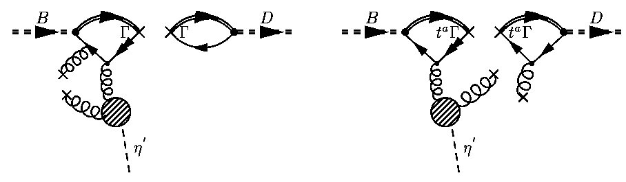 Figure 1
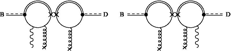 Figure 2
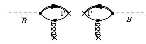 Figure 3
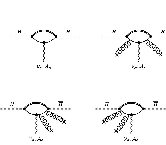 Figure 4
Peer Reviews
No public reviews on file for this paper yet. If you reviewed it on a platform where reviews are public (OpenReview, ICLR, NeurIPS, ICML), you can paste yours below so the community can read it here.
Videos
No videos yet. Explain this paper in a talk, walkthrough, or lecture? Add one.
Taxonomy
TopicsQuantum and electron transport phenomena · Advancements in Semiconductor Devices and Circuit Design · Quantum Computing Algorithms and Architecture
Low Energy Aspects of Heavy Meson Decays .††thanks: Presented at the Euridice meeting in Kazimierz, Poland, 24-27th of
august 2006
Jan O. Eeg
Department of Physics, University of Oslo,
P.O.Box 1048 Blindern, N-0316 Oslo, Norway
Abstract
I discuss low energy aspects of heavy meson decays, where there is at least one heavy meson in the final state. Examples are mixing, , , and . The analysis is performed in the heavy quark limit within heavy-light chiral perturbation theory. Coefficients of suppressed chiral Lagrangian terms (beyond factorization) have been estimated by means of a heavy-light chiral quark model.
\PACS
PACS numbers 13.20.Hw , 12.39.St , 12.39.Fe , 12.39.Hg
1 Introduction
In this paper we consider non-leptonic “heavy meson to heavy meson(s)” transitions, for instance -mixing [1], [2] and with only one -meson in the final state, like [3] and [4, 5, 6].
The methods [7] used to describe heavy to light tansitions like and are not suited for the decays we consider. We use heavy-light chiral perturbation theory (HLPT). Lagrangian terms corresponding to factorization are then determined to zeroth order in , where is the mass of the heavy quark ( or ). For -mixing we have also calculated corrections [1].
Colour suppressed terms beyond factorization can be written down, but their coefficients are unknown. However, these coefficients can be calculated within a heavy-light chiral quark model (HLQM) [8] based on the heavy quark effective theory (HQEFT) [9] and HLPT [10]. The suppressed non-factorizable terms calculated in this way will typically be proportional to a model dependent gluon condensate [1, 2, 3, 6, 8, 11].
2 Quark Lagrangians for non-leptonic decays
The effective non-leptonic Lagrangian at quark level has the form [12]:
[TABLE]
where the Wilson coefficients contain and KM factors. Typically, the operators are four quark operators being the product of two currents:
[TABLE]
where , and some of the quarks are heavy. To leading order in , matrix elements of factorize in products of matrix elements of currents. Non-factorizable suppressed terms are obtained from “coloured quark operators”. Using Fierz transformations and
[TABLE]
where are colour matrices, we may rewrite the operator as
[TABLE]
where is a left-handed coloured current. The quark operators in give suppressed terms.
3 Heavy-light chiral perturbation theory
The QCD Lagrangian involving light and heavy quarks is:
[TABLE]
where are the quark fields for a heavy quark and a heavy anti-quark with velocity , is the light quark triplet, and . The bosonized Lagrangian have the following form, consistent with the underlying symmetry [10]:
[TABLE]
where the covariant derivative is ; being SU(3) flavour indices. The axial coupling is . Furthermore,
[TABLE]
where , and is a 3 by 3 matrix containing the light mesons (), and the heavy doublet field is
[TABLE]
where superscripts means meson and anti-meson respectively. To bosonize the non-leptonic quark Lagrangian, we need to bosonize the currents. Then the , , and quarks are treated within HQEFT, which means the replacements , and . Then the bosonization of currents within HQEFT for decay of a heavy -meson will be:
[TABLE]
where is the left-handed projector in Dirac space, and for before pQCD and chiral corrections are added. Here, represents the heavy meson (doublet) containing a -quark. For creation of a heavy anti-meson or , the corresponding currents and are given by (9) with replaced by and , repectively. For the transition we have
[TABLE]
where is the Isgur-Wise function, and . For creation of pair we have the same expression for the current with replaced by , and replaced by , where . In addition there are corrections for . The low velocity limit is . For and one has and , respectively.
3.1 Factorized lagrangians for non-leptonic processes
For mixing, the factorized bosonized Lagrangian is
[TABLE]
where is a short distance Wilson coefficient (containing ), which is taken at 1 GeV, and the currents are given by (9).
For processes obtained from two different four quark operators for , we find the factorized Lagrangian corresponding to Fig. 1:
[TABLE]
where , and [13] , . We have considered the process . Note that there is no factorized contribution to this process if both -mesons in the final state are pseudoscalars! But the factorized contribution to will be the starting point for chiral loop contributions to the process .
The factorizable term from annihilation is shown in Fig. 2, and is:
[TABLE]
Because is a non-favourable combination of the Wilson coefficients, this term will give a small non-zero contribution if at least one of the mesons in the final state is a vector.
3.2 Possible suppressed tree level terms
For mixing, we have for instance the suppressed term
[TABLE]
For , we have for instance the terms
[TABLE]
[TABLE]
One needs a framework to estimate the coefficients of such terms. We use the HLQM, which will pick a certain linear combination of terms.
3.3 Chiral loops for non-leptonic processes
Within HLPT, the leading chiral corrections are proportional to
[TABLE]
where is the appropriate light meson mass and is the chiral symmetry breaking scale, which is also the matching scale within our framework.
For mixing there are chiral loops obtained from (6) and (11) shown in Fig. 3. These have to be added to the factorized contribution.
For the process we obtain a chiral loop amplitude corresponding to Fig. 4. This amplitude is complex and depend on and defined previously. It has been recently shown [5] that states in loops should also be added to the result.
4 The heavy-light chiral quark model
The Lagrangian for HLQM [8] contains the Lagrangian (5):
[TABLE]
where is the heavy quark part of (5), and the light quark part is
[TABLE]
Here and are flavour rotated light quark fields, and is the light constituent mass.
The bosonization of the (heavy-light) quark sector is performed via the ansatz:
[TABLE]
The coupling is determined by bosonization through the loop diagrams in Fig 6. The bosonization lead to relations between the model dependent parameters , , and , and the quadratic-, linear, and logarithmic- divergent integrals , and the physical quantities , , and ().
For example, the relation obtained for identifying the kinetic term is:
[TABLE]
where we have used the prescription:
[TABLE]
The parameters are fitted in strong sector, with GeV] and , where . For details , see [8].
5 terms from HLQM
To obtain the terms for mixing in Fig. 7 , we need the bosonization of colored current in the quark operators of eq. (4):
[TABLE]
[TABLE]
This coloured current is also used for in Fig. 8, for in Fig. 9, and for in Fig. 10 In addition there are more complicated bosonizations of coloured currents as indicated in Fig. 8.
For and decays there are two different four quark operators, both for and , respectively. At GeV they have Wilson coefficients (up to prefactors and KM-factors).
For , we must also attach a propagating gluon to the -vertex. Note that for , the suppressed mechanism in Fig. 10 dominates, unlike . Factorized contributions are proportional to either the favourable contribution or the non-favourable contribution .
5.1 correction terms
For the transition we have the suppressed terms:
[TABLE]
where the ’s are calculable within HLQM. The relative size of corrections are typically of order .
6 Results
6.1 mixing
The result for the B(ag) parameter in -mixing has the form [1]
[TABLE]
similar to the -mixing case [11]. From perturbative QCD we have at = 1 GeV. From calculations within the HLQM we obtain, and GeV, and from chiral corrections GeV2, and GeV2. We obtained
[TABLE]
in agreement with lattice results.
6.2 decays
Keeping the chiral logs and the terms from the gluon condensate, we find the branching ratios in the “leading approximation”. For decays of () and () we obtain branching ratios of order few and , respectively Then we have to add counterterms for chiral loops. These may be estimated in HLQM.
6.3 and
decays
The result corresponding to Fig. 9 is:
[TABLE]
The partial branching ratios from the mechanism in Fig. 10 are [6]
[TABLE]
The corresponding factorizable contribibutions are roughly two orders of magnitude smaller. Note that the process has substantial meson exchanges (would be chiral loops for ), and is different.
7 Conclusions
Our low energy framework is well suited to mixing, and to some extent to . Work continues to include , states, counterterms, and terms. Note that the amplitude for is zero in the factorized limit. For processes like and we can give order of magnitude estimates when factorization give zero or small amplitudes.
JOE is supported in part by the Norwegian research council and by the European Union RTN network, Contract No. HPRN-CT-2002-00311 (EURIDICE). He thanks his collaborators : A. Hiorth, S. Fajfer, A. Polosa, A. Prapotnik Brdnik, J.A. Macdonald Sørensen, and J. Zupan
The reference list from the paper itself. Each links out to its DOI / PubMed record.
- 1[1] A. Hiorth and J. O. Eeg, Eur. Phys. J. direct C 30 , 006 (2003) (see also references therein).
- 2[2] J.O. Eeg, S. Fajfer , and A. Hiorth, Phys.Lett. B 570 , 46-52 (2003); J. O. Eeg, S. Fajfer, and A. Prapotnik Eur. Phys. J. C 42 , 29-36 (2005). See also: J.O. Eeg, S. Fajfer, J. Zupan, Phys. Rev. D 64 , 034010 (2001).
- 3[3] J. O. Eeg, A. Hiorth, A. D. Polosa, Phys. Rev. D 65 , 054030 (2002).
- 4[4] B.Grinstein and R.F. Lebed, Phys.Rev. D 60 , 031302(R) (1999).
- 5[5] O. Antipin and G. Valencia, Phys.Rev. D 74 , 054015 (2006), hep-ph/0606065.
- 6[6] J.A. Macdonald Sørensen and J.O. Eeg, hep-ph/0605078.
- 7[7] M. Beneke et. al , Phys. Rev. Lett. 83 , 1914 (1999); C. W. Bauer et al. Phys. Rev. D 70 , 054015 (2004)
- 8[8] A. Hiorth and J. O. Eeg, Phys. Rev. D 66 , 074001 (2002), and references therein.