Towards self-consistent definition of instanton liquid parameters
S.V. Molodtsov, G.M. Zinovjev

TL;DR
This paper explores a self-consistent approach to defining instanton liquid parameters, focusing on optimal pseudo-particle configurations and the effects of interactions within the ensemble.
Contribution
It introduces a method for self-consistently determining instanton liquid parameters and compares different pseudo-particle ensemble configurations.
Findings
Weakening of repulsive interactions between pseudo-particles is estimated.
Optimal pseudo-particle configurations are identified.
A framework for self-consistent parameter determination is proposed.
Abstract
The possibility of self-consistent determination of instanton liquid parameters is discussed together with the definition of optimal pseudo-particle configurations and comparing the various pseudo-particle ensembles. The weakening of repulsive interactions between pseudo-particles is argued and estimated.
Click any figure to enlarge with its caption.
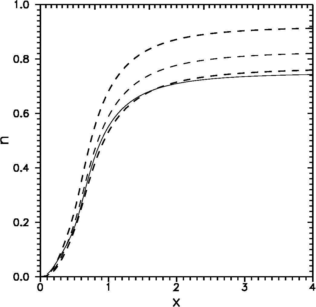 Figure 1
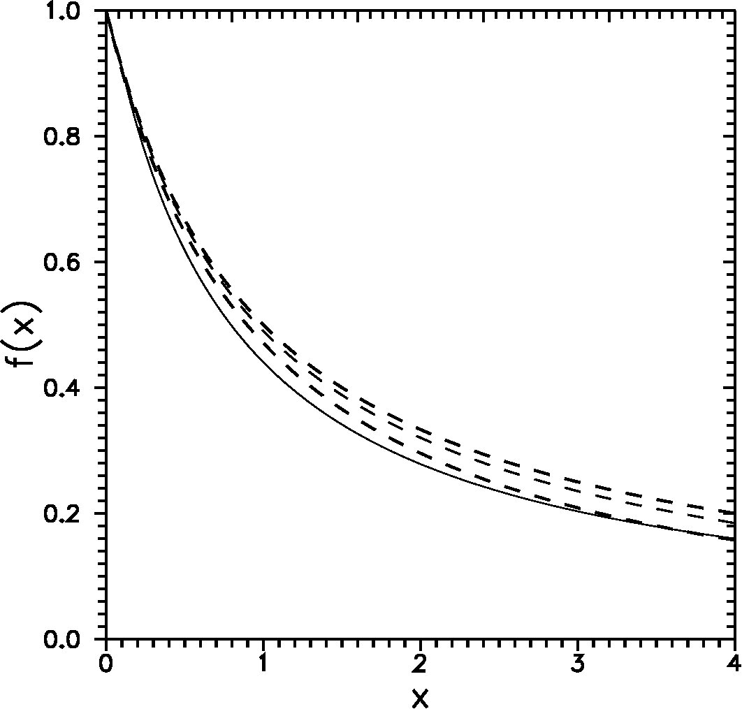 Figure 2
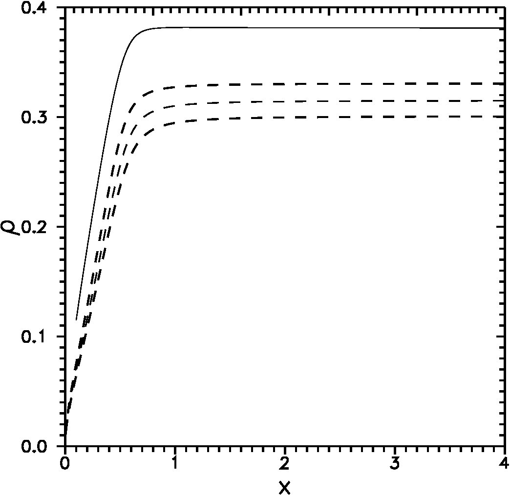 Figure 3
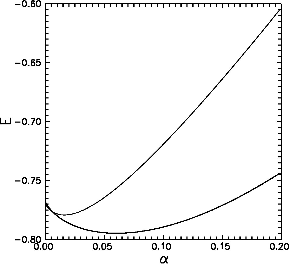 Figure 4
Peer Reviews
No public reviews on file for this paper yet. If you reviewed it on a platform where reviews are public (OpenReview, ICLR, NeurIPS, ICML), you can paste yours below so the community can read it here.
Videos
No videos yet. Explain this paper in a talk, walkthrough, or lecture? Add one.
**Towards self-consistent definition of instanton liquid parameters
** S.V. Molodtsov1,2, G.M. Zinovjev3
1Joint Institute for Nuclear Research, RU-141980, Dubna, Moscow region, Russia
2Institute of Theoretical and Experimental Physics, RU-117259, Moscow, Russia
3Bogolyubov Institute for Theoretical Physics, National Academy of Sciences of Ukraine, UA-03680, Kiev-143, Ukraine
[TABLE]
The problem of finding the most effective pseudo-particle profile for instanton liquid (IL) model of the QCD vacuum [1] has already been formulated in the first papers treating the pseudo-particle superposition as the quasi-classical configuration saturating the generating functional [2] of the following form
[TABLE]
where is the Yang-Mills action. Although the solution proposed in Ref. [2] was quite acceptable phenomenologically the consequent more accurate analysis discovered several imperfect conclusions putting into doubt the assertion about the instanton ensemble getting stabilization and some additional mechanism should be introduced to fix such an ensemble [3]. In this note we revisit the task formulated in Ref. [2] within the self-consistent approach proposed in our previous paper [4]. We are not speculating on the detailed mechanism of stabilizing and are based on one crucial assumption which is the existence of non-zero gluon condensate in the QCD vacuum. This idea is not very original but turns out far reaching in the context of our approach. The particular form and properties of this condensate will be discussed in the following paper.
Thus, as the configuration saturating the generating functional (1) we take the following superposition
[TABLE]
here stands for the (anti-)instanton field in the singular gauge
[TABLE]
denotes all the parameters describing the -th (anti-)instanton, in particular, its size , colour orientation , center position and as usual is the coupling constant of gauge field. The function introduces the pseudo-particle profile and will be fixed by resolving the suitable variational problem. For example, for the conventional singular instanton it looks like
[TABLE]
In analogy with this form we consider the function depending on or, more precisely, on the variable at some characteristic mean pseudo-particle size . Dealing with the anti-instanton one should make the substitution of the ’t Hooft symbol . It is seen from (2) we ’singled out’ one pseudo-particle of ensemble and introduced the special symbol for its field which actually has the same form as Eq. (3).
The strength tensor of this ’external’ field and the field of every separate pseudo-particle can be written as
[TABLE]
where two first terms are given by the standard definition of field strength
[TABLE]
with the entirely antisymmetric tensor . In particular, for the singular instanton of Eq. (3) it takes the form
[TABLE]
where means the derivative over . The third term of Eq. (5) presents the ’mixed’ component of field strength and is
[TABLE]
It was shown in Ref. [4] that in quasi-classical regime which is of particular interest for applications, the generating functional (1) could be essentially simplified if reformulated in terms of the field averaged over ensemble . Performing the cluster decomposition [5] of stochastic exponent in Eq. (1)
[TABLE]
where , (the first cumulant is simply defined by averaging the action) the higher terms of effective action for the ’external’ field in IL could be presented as
[TABLE]
and the mass is defined by the IL parameters developing for the standard singular pseudo-particles (4) the following form (see, also below)
[TABLE]
with where is the total number of pseudoparticles in the volume and is the number of colours. The small magnitude of characteristic IL parameter (packing fraction) allows us at decomposing to keep the contributions of one pseudo-particle term () only.
The effective action in Eq. (10) implies a functional integration in which the vacuum stochastic fields are not destroyed by the external field. Then there is no reason to develop the detailed description of the field driven by the symmetries of initial gauge invariant Lagrangian for the Yang-Mills fields. In practice it could be understood as an argument to do use the averaged action dealing with the field . It means the colourless binary (and similar even) configurations only of field survive in the effective action. In other words the decomposition is used (in what follows we are not maintaining the index for the field ). Obviously, if there is any need of more detailed description including, for example, information on the fluctuations of field one should operate with the correlation functions of higher order and the corresponding chain of the Bogolyubov equations.
The selfconsistent description of pseudo-particle ensemble may not be developed based on Eq. (10) only because in such a form the pseudo-particles of zero size are most advantageous. In Ref. [4] the version of variational principle was proposed which makes it possible to determine the selfconsistent solution in long wave-length approximation for the pseudo-particle ensemble (anti-instantons in the singular gauge with standard profile (4)) and external field. Here it adapts to the saturating configuration (2) also and its more optimal (than standard) profile is defined, as suggested in Ref. [2], taking into account the IL parameter change while the pseudo-particle field is present.
The contribution of saturating configuration into the generating functional is evaluated as (see [2] for the denotions)
[TABLE]
The following terms should be taken into consideration
[TABLE]
(the details of deducing this expression can be found in [4]). Here we remind only that to obtain it one should average over the pseudo-particle parameters and to hold the highest contributions only at summing up the pseudo-particles. If the saturating configurations are the instantons in singular gauge with the standard profile (4) the first term describing the one instanton contributions takes the form of distribution function over (anti-)instanton sizes
[TABLE]
where
[TABLE]
,
[TABLE]
If one considers the profile of Eq. (3) the change of one pseudo-particle action which has the form
[TABLE]
should be absorbed while calculating. Here is the characteristic action of single pseudo-particle (4) which is defined at the scale of average pseudo-particle size where . The coefficient enters the corresponding equations (in particular the distribution function (14)) always with the additional factor . It means that in all the formula containing the one instanton contribution the following substitution
[TABLE]
should be done. The penultimate term of Eq. (13) accumulates the partial pseudo-particle contributions coming from the ’mixed’ component of the strength tensor (8) and describing the interaction of pseudo-particle ensemble with the detached one, i.e.
[TABLE]
The other terms at the characteristic IL parameters are small as it was shown in Ref. [4]. The average value of ’mixed’ component is given by the following formula
[TABLE]
here is defined by the integrated profile function of pseudo-particle
[TABLE]
In particular, for the standard form of pseudo-particle we have
[TABLE]
The corresponding constant (see [4]) should be changed for the modified one
[TABLE]
in all terms describing the interaction of IL with detached pseudo-particle if the profile function is arbitrary. Eq. (18) demonstrates that we are formally dealing with non-zero value of gluon condensate which is given by the correlation function
[TABLE]
For the pseudo-particle of standard form the function equals to
[TABLE]
with the asymptotic behaviours
[TABLE]
The presence of this condensate (19) which leads, in particular, to the mass definition as in (11) just signifies the assumption mentioned at the beginning this note.
The second term of (13) describes the repulsive interaction between the pseudo-particles of ensemble
[TABLE]
and actually presents the same contribution as but being integrated with the field of every individual pseudo-particle as . It results in the change of coupling constant describing the pseudo-particle interaction (see [2]) for new form
[TABLE]
(similar to the change of constant ). And eventually the last term of Eq. (13) presents simply the Yang-Mills action of the field
[TABLE]
It is worthwhile to notice that the topological charge of the configuration (4) is retained to be equal to
[TABLE]
here is an entirely antisymmetric tensor, .
The generating functional (12) might be estimated with the approximating functional (see [2]) as
[TABLE]
where
[TABLE]
and is an effective one particle distribution function defined by solving the variational problem. In our particular situation the average value of difference of the actions is given as follows
[TABLE]
with . In this note we estimate the functionals in the long wave length (adiabatic) approximation, i.e. consider the IL elements to be equilibrated by the external fixed field . Afterwards, with finding the optimal IL parameters out we receive the effective action for the external field in the selfconsistent form. Eq. (S0.Ex14) is taken just in such a form in order to underline the integration is executed over the IL elements and the parameters describing their states are the functions of external field (i.e. could finally be the functions of a coordinate x). The physical meaning of such a functional is quite transparent and implies that each separate IL element develops its characteristic screening of the attached field.
Now calculating the variation of action difference over we obtain
[TABLE]
where is an arbitrary constant and its value is fixed by requiring the coincidence of the distribution function when the external field is switched off () with vacuum distribution function then
[TABLE]
With defining the average size as
[TABLE]
we come to the practical interrelation between the IL density and average size of pseudo-particles
[TABLE]
where . Apparently, the size distribution of pseudo-particles can be presented by the well-known form as
[TABLE]
Eqs. (S0.Ex14) and (25) allow us to get the estimate of generating functional (21) in the following form
[TABLE]
[TABLE]
Now taking into account Eq. (24) and fixing a field , parameters and the maximum of functional (26) over the IL parameters can be calculated by solving the corresponding transcendental equation () numerically. Here it is a worthwhile place to notice the presence of new factor in the denominator of what is caused by the Gaussian form of the corresponding integral over squared and, hence, the integration element requires the introduction of . In Ref. [2] this factor was missed. However, this fact has not generated a serious consequence because any application of these results is actually related to the choice of suitable quantity of the parameter entering the observables (the pion decay constant, for example). It means we should make the proper choice of basic scale. Besides, we should also keep in mind the approximate character of IL model. Further we give the results for both versions to demonstrate the dependence of final results on the renormalized constant .
Searching the optimal configuration we take the effective action in the form of nonlinear functional as
[TABLE]
in which the IL state is described by solutions , . In practice the following differential equation should be resolved
[TABLE]
at fixed initial magnitude of putting up the derivative in the initial point in such a way to have the solution going to zero when x is going to infinity. Parameter is introduced to fix a priori unknown value of coupling constant in the pseudo-particle definition (3). If the profile function has been fixed the configuration should be found in the form in which the starting values of parameters , and coincide (within the given precision) with the parameters obtained from the solution . Nowadays this approach looks the most optimal one among other existing possibilities not only because of the computational arguments but in view of the poor current level of understanding the interrelation between perturbative and non-perturbative contributions while calculating the effective Lagrangian. In fact, it was mentioned in Ref. [2] that in more general (realistic) formulation of this problem Eq. (28) should include the term responsible for the change of ’quantum’ constant with the function changing. In principle, it could imply that the problem of pseudo-particle ensemble stabilization is connected at the fundamental dynamics level with the anticipated smallness of the contribution and, apparently, should be addressed not so much to the description of the interacting pseudo-particles and their interactions with the perturbative fields but rather to investigation of the time hierarchy corresponding to the breakdown of quasi-stationary behaviour of the vacuum fluctuations which will certainly lead to the changes of suitable effective Lagrangian (10).
In order to receive the preliminary parameter estimates we consider the simplified model with the profile function containing only one additional parameter for describing the screening effect as regards
[TABLE]
The energy as the function of the screening parameter is depicted in Fig. 1. The lowest dashed curve shows the behaviour when the changes related to weakening of repulsive interaction are taken into account by switching on the parameter only (at ). The top dashed curve was obtained with both parameters switched on. The optimal value of the screening parameter is determined by the minimum point of function . Besides, this figure demonstrates the stability of variational procedure of extracting the IL parameters. For the first calculation the values of characteristic parameters for corresponding solution were taken as , , with the following set of the IL parameters , , . These values give for the ratio of average pseudo-particle size and average distance between pseudo-particles the quite suitable quantity . For another calculation we have treated the parameter set characterizing the solution as , , and for the IL parameters the following values , , , . In order to get more orientation we would like to mention that for the ensemble of standard pseudo-particles (, , ) the corresponding values are , , , .
Now we examine the impact of correction introduced in Eq. (26) when we changed the term which has been obtained in Ref. [2]. For the first calculation with the set of solution parameters as , , we have for the IL parameters , , which lead to the ratio discussed equal to . For another calculation we have the following results , , and , , , . And for the ensemble of standard pseudo-particles (, , ) these parameters are , , , .
The Fig. 2 and Fig. 3 show the behaviours of IL density and average pseudo-particle size as the functions of distance . The dashed lines on both plots correspond to the similar ensembles. The lowest curves demonstrate the behaviours for the ensembles of standard pseudo-particles (4). The top curves present the ensemble of pseudo-particles with the profile function (29) at and . And the middle dashed lines correspond to the profile functions with and . Obviously, it may be concluded that including even small change of the second parameter value () leads to the noticeable change of ensemble characteristics (for example, the IL density) because the highest contribution to the action when the coupling constant becomes the function of is essentially modified.
Let us make now several comments as to the ’complete’ formulation of the problem of analyzing the equation (28). It was numerically resolved by the Runge-Kutta method. This approach combined with numerical calculation of the derivative at every point of consequent integration interval allows us to avoid the problems which appear when searching the minimum of complicated functional in multidimensional space.
The initial data were fixed at the point . Since the IL density value at the coordinate origin is inessential the initial form of pseudo-particle profile function is taken without any deformations as . Then at fixed values of the parameters , and the coefficient is calculated. It allows to set the slope of trajectory at initial point in such a form in order to have the solution going to zero at large distances. Afterwards we find out the values of parameters and requiring the input data to coincide with the output ones within the fixed precision. The parameter values which obey the imposed constraints are the following (input values) , , at and , , (at the output of variational procedure). The solid line in Fig. 4 shows the obtained profile as the function of . The differences of profiles are smoothed over if they are presented as the functions of because the large magnitude of the screening coefficient, for example , is compensated by enlargening the pseudo-particle size. The dashed lines on this plot show the profile functions for the standard form (4) (top dashed line), with the screening factor (29) including one parameter only () (lowest dashed curve) and two parameters included (middle dashed line).
Another calculation (with modified -function contribution) was based on the slightly different set of relevant parameters which are for the input values , , at and , , for the output one at the finish of variational procedure. The behaviours of IL density and average pseudo-particle size for selfconsistent solution are plotted in Fig. 2 and Fig. 3 (solid lines, respectively)111It is interesting to notice that considering IL (ensemble of pseudo-particles in the singular gauge) in the field of regular pseudo-particle we obtain the IL density value in the center of regular pseudo-particle which is larger than its value at large distances what looks like the anti-screening effect.. In the Table 1 we present the IL parameters at the large distances from pseudo-particle (the first line) together with the data for the ensemble of pseudo-particles with the standard profile function (the second line). The third and fourth lines of this Table 1 are devoted to the calculations with the second set of parameters (with factor absent in Eq. (26)). The fourth line, in particular, presents the calculations for pseudo-particles with standard form of profile function.
Table 1. Parameters of IL.
[TABLE]
It is quite obvious that the utilization of optimal pseudo-particle profile function leads to the larger pseudo-particle size but the packing fraction parameter holds, nevertheless, a small quantity which is quite suitable for the perturbative expansion. Besides, the results obtained allow us to conclude that with tuning a fully satisfactory agreement our calculations of pseudo-particle size, the ensemble diluteness and gluon condensate value with their phenomenological magnitudes extracted from the other models are easily reachable. The calculations of several dimensional quantities in our approach are also very indicative. The values of the screening mass (11), average pseudo-particle size and IL density obtained for two values of ( MeV and MeV) are shown in Table 2. The sequence of line meanings is identical to that in Table 1 as well as the meanings of last four lines which present the results of calculations with the second set of parameters (with factor absent in Eq. (26)).
Table 2. Screening mass and IL parameters
[TABLE]
Another interesting feature of this calculation is the weakening of pseudo-particle interaction. This effect is driven by the coefficient (). Our estimates for the first set of parameters give and, hence, and for the second set we have () and . Let us mention here that the reasonable description of instanton ensemble can be reached in the framework of two-component models [6] as well.
Our calculations enable us to conclude that dealing with IL model (formulated in one-loop approach) one is able to reach quite reasonable description of gluon condensate even being constrained by the values of average pseudo-particle size and other routine phenomenological parameters. Moreover, the ensemble of pseudo-particles with standard profile functions turns out to be very practical because introducing the other configurations to make the similar estimates is simply unoperable. With such an approximation of the vacuum configurations the coefficient of interaction weakening develops the magnitude about — . Including this effect leads to the enlargening of pseudo-particle size. It allows us to conclude that nowadays the instantons in the singular gauge is the only serious instrument for effective practising.
The authors are sincerely grateful to A.E. Dorokhov and S.B. Gerasimov for interesting discussions and practical remarks. The financial support of the Grants INTAS-04-84-398 and NATO PDD(CP)-NUKR980668 is also acknowledged.
The reference list from the paper itself. Each links out to its DOI / PubMed record.
- 1[1] C.G. Callan, R. Dashen, and D.J. Gross, Phys. Lett. B 66 (1977) 375; C.G. Callan, R. Dashen, and D.J. Gross, Phys. Rev. D 17 , (1978) 2717.
- 2[2] D.I. Diakonov and V.Yu. Petrov, Nucl. Phys. B 245 , (1984) 259.
- 3[3] I.I. Balitsky and A.V. Yung, Phys. Lett. B 168 , (1986) 113; D. Förster, Phys. Lett. B 66 , (1977) 279; E.V. Shuryak and J.J.M. Verbaarschot, Nucl. Phys. B 364 , (1991) 255; T. Schäfer and E.V. Shuryak, Rev. Mod. Phys. 70 , (1998) 323.
- 4[4] S.V. Molodtsov, G.M. Zinovjev, Yad. Fiz. 70 , 𝒩 𝒩 \cal N 0 6 , (2007).
- 5[5] N.G. Van Kampen, Phys. Rep. 24 (1976) 171; Physica 74 (1974) 215, 239; Yu.A. Simonov, Phys. Lett. B 412 (1997) 371.
- 6[6] A.E. Dorokhov, S.V. Esaibegyan, A.E. Maximov, and S.V. Mikhailov, Eur. Phys.J C 13 (2000) 331; N.O. Agasian and S.M. Fedorov, JHEP 12 (2001) 019.